11  Decision Trees

It is now time to introduce a second model architecture. How would you predict the class of the unknown observation without using distance functions or nearest neighbours?

New observation and example data

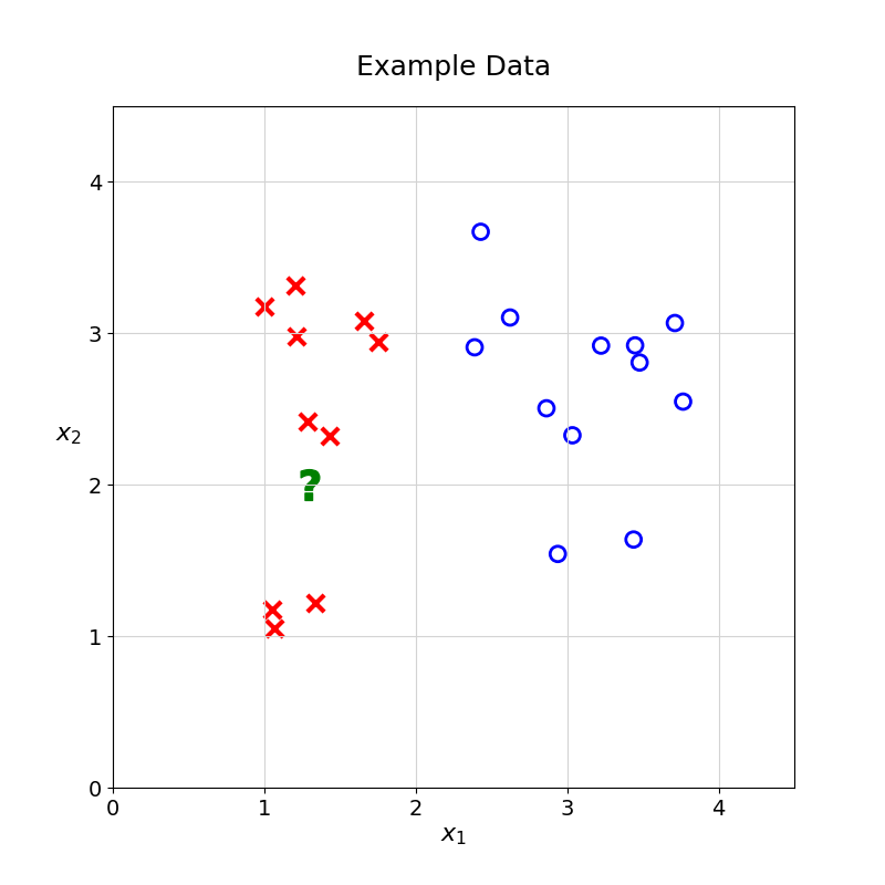
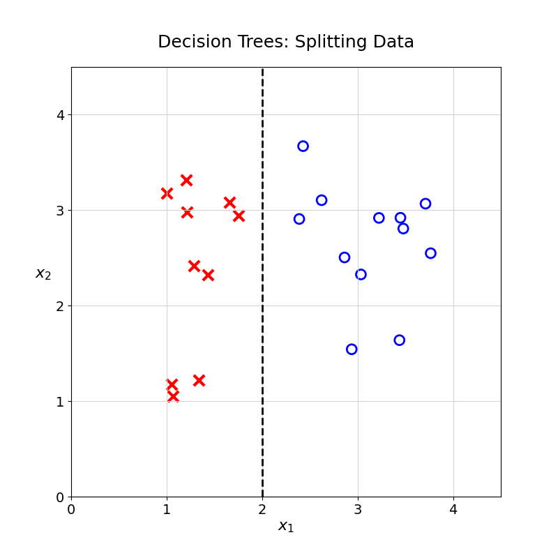
One possibility would be to split the data at \(x_1 = 2\). Any observation with \(x_1\) greater than \(2\) would be classified as \(\circ\); the rest would be classified as \(\times\).

Example data with a single split

11.1 Multiple Splits

For a more complex case, how would you predict the class of the unknown observation with this training data? How would you split the \(\times\) from the \(\circ\)?

A more complex example problem

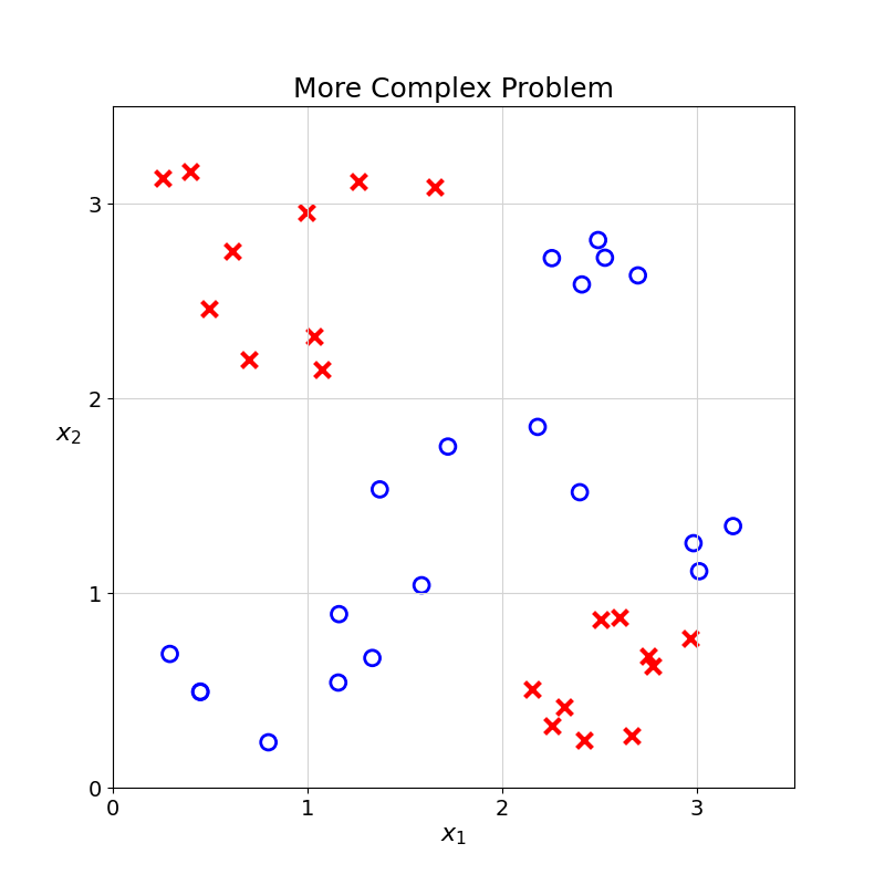
In this example, there is no single line that can perfectly split the two groups. In Computer Science, this is also called the XOR problem.

NoteXOR Problem

The XOR (Exclusive Or) Problem refers to a foundational Machine Learning and Computer Science problem in which two classes cannot be separated by any single straight line. It demonstrates the weaknesses of simple linear models.

XOR Problem: Can you find a single line separating the x from the o?

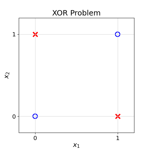
The XOR is a logical operation that takes two Boolean (True/False or 1/0) values as inputs and returns 1 (or True) if they are different and 0 or False otherwise. You can see the truth table for this operation below.

XOR Truth Table

Input A	Input B	Output (A XOR B)
False	False	False
False	True	True
True	False	True
True	True	False

More information on the XOR problem at (“Exclusive Or,” n.d.)

Instead of splitting the data once, what if you could split the data multiple times? An example is shown below:

Splitting the data multiple times

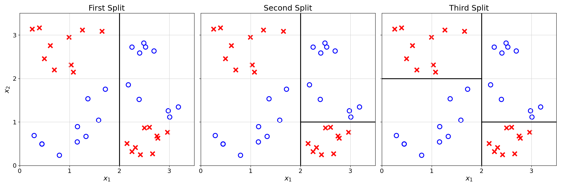
11.2 From Splits to Predictions

Using these three splits, how could you classify a new observation?

One way to do so would be to go through the splits we did one by one:

• If \(x_1 \geq 2\):
  • If \(x_2 \geq 1\): assign \(\circ\)
  • Else: assign \(\times\)
• Else:
  • If \(x_2 \geq 2\): assign \(\times\)
  • Else: assign \(\circ\)

The observation is then assigned the label that is the majority in the resulting partition.

Exercise 11.1 Using the above list, generate predictions for the following observations:

• Observation 1: \(x_1 = 3,x_2 = 3\)
• Observation 2: \(x_1 = 1,x_2 = 3\)
• Observation 3: \(x_1 = 1,x_2 = 1\)

11.3 From Partition to Trees

The above list may be difficult to follow. This type of logic could be more elegantly represented as a tree (also called a decision tree):

Visualising splits as a Decision Tree

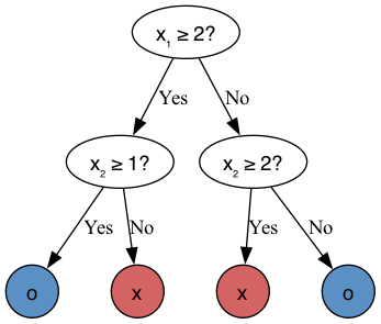
Exercise 11.2 Generate predictions for the following observations by going down the Decision Tree above:

• Observation 1: \(x_1 = 3,x_2 = 3\)
• Observation 2: \(x_1 = 1,x_2 = 3\)
• Observation 3: \(x_1 = 1,x_2 = 1\)

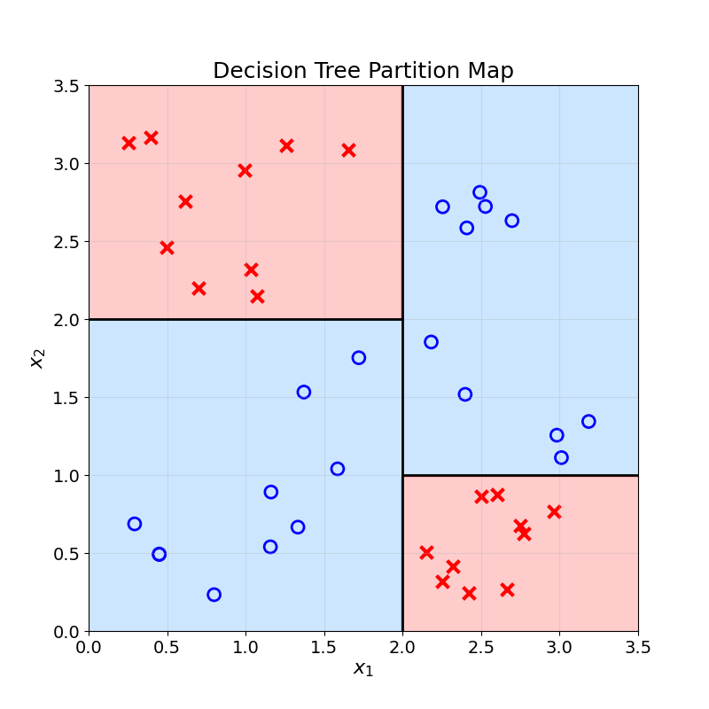
To better understand the relationship between trees and data splits, the tree and the partition can be visualised next to one another:

Decision Tree as a partition of space

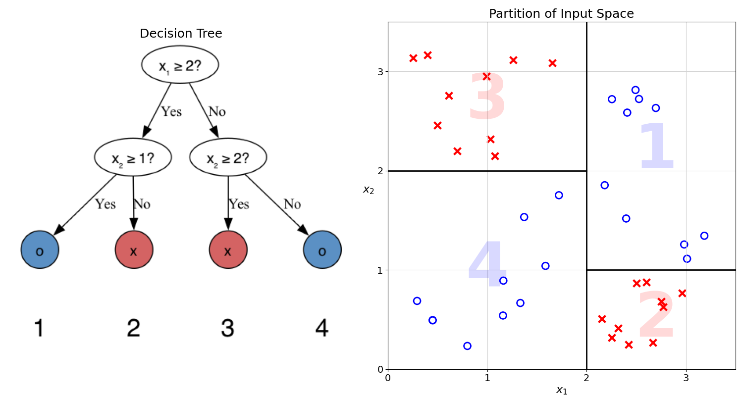
Each split or comparison creates a linear separation in the feature space, represented by a black line in the chart above.

In Computer Science, trees are a type of graph. Graphs are collections of nodes and edges.

Graphs are collections of nodes and edges connecting them

Edges can be directed or undirected. Directed edges can only be traversed in one direction, usually represented as arrows. Edges, i.e., connections between nodes, can form cycles. These cycles are paths that start and end with the same node.

Edges can be directed

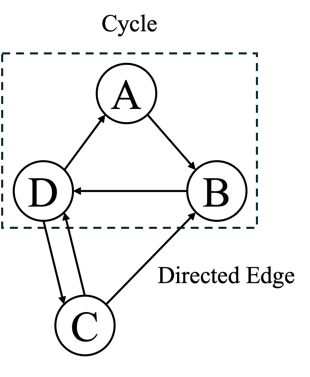
Exercise 11.3 The diagram above highlights the cycle A→B→D→A. Can you find another cycle?

Trees are Directed Acyclic Graphs (DAGs). This is a bit of a mouthful, let’s take these terms one by one:

• Directed: They flow from the root to the leaves
• Acyclic: They do not contain any cycles; there is only a single path from the root to each node

Below is an example of a tree with seven nodes:

A simple tree with seven nodes

Trees, like all graphs, are composed of nodes and edges. In addition to the usual graph jargon, there are a few tree-specific concepts. To understand them, consider the example above:

• Parent and child nodes: both connected by an edge (nodes B and D)
• Root node: The topmost node of a tree (node A)
• Leaf node: A node with no children (node G)

Exercise 11.4 Find another example of:

• Leaf node
• Parent node

11.4 From Trees to Maps

Just like the KNN model, Decision Trees build a map from the input features to the target variable. Using a Decision Tree to generate predictions for all possible feature values, we get the following map:

Building a map with Decision Trees

11.5 Final Thoughts

That is it, we have built our first Decision Tree! We can use this model to predict any new observation based on its two features and position on the map above.

This is only a simple introduction to Decision Trees. The next chapters will explore the inner workings of this model family, starting with the evaluation of data splits. What makes a good split of a dataset?

11.6 Solutions

Solution 11.1. Exercise 11.1

• Observation 1: \(\circ\)
• Observation 2: \(\times\)
• Observation 3: \(\circ\)

Solution 11.2. Exercise 11.2

• Observation 1: \(\circ\)
• Observation 2: \(\times\)
• Observation 3: \(\circ\)

Solution 11.3. Exercise 11.3 There are many possible cycles, here are two examples:

• C→D→C
• C→B→D→C

Exercise 11.5 Solution. Exercise 11.5

• Leaf node: D, E, F, G
• Parent node: A, B, C

“Exclusive Or.” n.d. https://en.wikipedia.org/wiki/Exclusive_or.