6 Computing Errors with Sigma Notation
The MAE and MSE calculations were both introduced with the dot notation (noted \(\cdots\)). For example:
\[ \text{MSE} = \frac{\text{Error}_1^2 + \text{Error}_2^2 + \cdots + \text{Error}_n^2}{n} \]
This is fine for a small number of terms, but there are more compact ways to deal with sums of large lists of numbers. This is what the Sigma operator is all about. It is a big scary Greek letter that the rest of this chapter will try to make less scary.
6.1 The Sigma Operator
The Sigma operator (\(\Sigma\)) is a summation operator. It represents the sum (or addition) of several terms. If we want to represent the sum of integers from 1 to 4, we can write it:
\[ 1 + 2 + 3 + 4 \]
Or with the Sigma operator:
\[ \sum_{i=1}^{4} i = 1 + 2 + 3 + 4 \]
What just happened? We had a nice friendly sum and now there is a \(\Sigma\), \(i\) and numbers flying around. Let’s break this formula down:
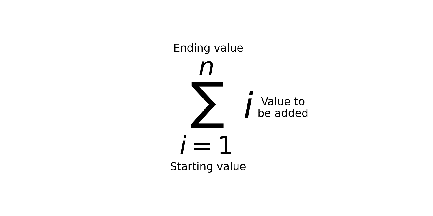
- \(i\) is the counter
- It starts at \(i = 1\), shown below the Sigma operator
- And ends at \(4\), shown on top of the Sigma operator
Whatever comes to the right of the \(\Sigma\) is the value to be added. Let’s start with an even simpler example:
\[ \sum_{i=1}^{3} 2 \]
Here, the counter starts at \(i = 1\) and ends at \(i = 3\). The value to be summed is the constant 2:
\[ \sum_{i=1}^{3} 2 = 2 + 2 + 2 = 6 \]
The constant 2 is added 3 times. What about the following example?
\[ \sum_{i=1}^{3} i \]
Here, \(i\) would be added 3 times. The value of \(i\) changes at each iteration. So we would get:
\[ \sum_{i=1}^{3} i = 1 + 2 + 3 = 6 \]
Nothing more complicated.
More generally, to represent the sum of integers from 1 to \(n\), we can write:
\[ \sum_{i=1}^{n} i = 1 + 2 + \cdots + (n-1) + n \]
Exercise 6.1 Compute the following:
- \(\displaystyle\sum_{i=2}^{4} 3\)
- \(\displaystyle\sum_{i=1}^{4} i\)
- \(\displaystyle\sum_{i=1}^{4} 2i\)
- \(\displaystyle\sum_{i=1}^{4} \frac{i}{2}\)
6.2 Applying Sigma to MAE and MSE
The same notation can be applied to the mean absolute error (MAE) and the mean squared error (MSE). To do so, each observation of the dataset is numbered from 1 to \(n\), with \(n\) the total number of observations.
Going back to the example data with line a:
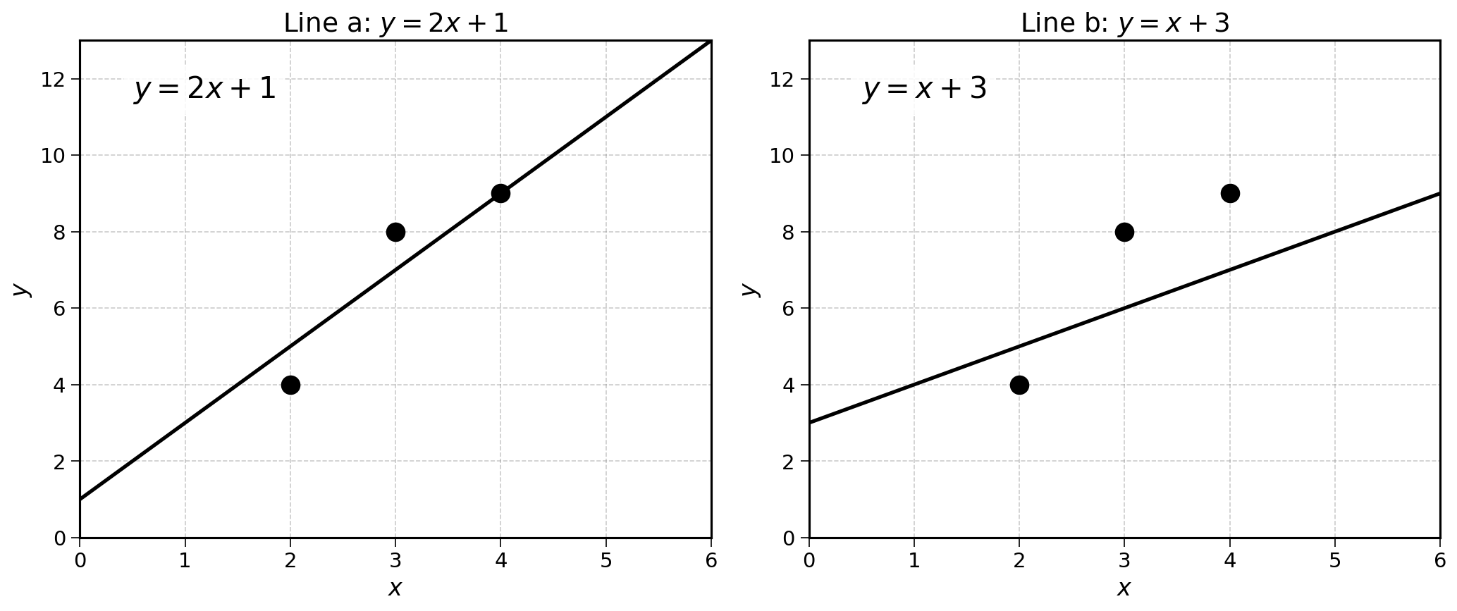
| \(i\) | \(y_i\) | Pred. (\(\hat{y}_i\)) | Error (\(\hat{y}_i - y_i\)) | \(|\text{Error}|\) | Error² |
|---|---|---|---|---|---|
| 1 | 4 | 5 | +1 | 1 | 1 |
| 2 | 8 | 7 | −1 | 1 | 1 |
| 3 | 9 | 9 | 0 | 0 | 0 |
Using Sigma notation, the MAE can be written as:
\[ \text{MAE} = \frac{1}{n} \sum_{i=1}^{n} |\hat{y}_i - y_i| \]
And the MSE as:
\[ \text{MSE} = \frac{1}{n} \sum_{i=1}^{n} (\hat{y}_i - y_i)^2 \]
These are equivalent to summing the errors (absolute value or squared) and dividing by the number of observations to get an average. The \(\hat{y}_i\) notation (read “y hat”) refers to the predicted value for observation \(i\).
Exercise 6.2 Compute the MAE and MSE of linear regression b (\(y = x + 3\)), showing that it is a worse model than linear regression a.
| \(i\) | \(x_i\) | \(y_i\) | Prediction (\(\hat{y}_i\)) | Error (\(\hat{y}_i - y_i\)) | \(|\text{Error}|\) | Error² |
|---|---|---|---|---|---|---|
| 1 | 2 | 4 | ||||
| 2 | 3 | 8 | ||||
| 3 | 4 | 9 |
6.3 Manipulating Expressions with the Sigma Operator
The mathematical rules that apply to sums also apply to the Sigma operator. For example, the distributive property states:
\[ a \times b + a \times c = a(b + c) \]
As a concrete example:
\[ 2 \times 1 + 2 \times 2 = 2(1 + 2) = 6 \]
Looking at this Sigma expression:
\[ \sum_{i=1}^{2} 2i = 2 \times 1 + 2 \times 2 = 2(1 + 2) \]
So far, so good. There is a deeper finding here. This means that we can take constants out of the Sigma operator:
\[ \sum_{i=1}^{2} 2i = 2 \sum_{i=1}^{2} i \]
This will be very useful going forward.
The MSE and MAE can be used to evaluate the accuracy of any predictive model, not just linear regressions. If you wanted to evaluate the accuracy of a weather forecast, you could calculate the Mean Squared Error of the temperature predictions:
\[ \text{MSE}_{\text{weather}} = \frac{1}{n} \sum_{i=1}^{n} (\text{Predicted Temperature}_i - \text{Actual Temperature}_i)^2 \]
The lower the MSE, the better the weather forecast.
6.4 Final Thoughts
Using the mean squared error and mean absolute error, we can evaluate the predictive accuracy of any line, on any dataset. This is already a lot. For ease of explanation, we will use the mean squared error (MSE) in the rest of this book.
The \(\Sigma\) notation is simply a more compact way to write sums. It is just a counter that adds things up.
Using these evaluation methods, the next chapter will explore how to find the regression lines that minimise the Mean Squared Error.
6.5 Solutions
Solution 6.1. Exercise 6.1
\(\displaystyle\sum_{i=2}^{4} 3 = 3 + 3 + 3 = 9\)
The counter goes from 2 to 4 (three iterations), and the constant 3 is added each time.
\(\displaystyle\sum_{i=1}^{4} i = 1 + 2 + 3 + 4 = 10\)
\(\displaystyle\sum_{i=1}^{4} 2i = 2(1) + 2(2) + 2(3) + 2(4) = 2 + 4 + 6 + 8 = 20\)
\(\displaystyle\sum_{i=1}^{4} \frac{i}{2} = \frac{1}{2} + \frac{2}{2} + \frac{3}{2} + \frac{4}{2} = 0.5 + 1 + 1.5 + 2 = 5\)
Solution 6.2. Exercise 6.2
For line b (\(y = x + 3\)):
| \(i\) | \(x_i\) | \(y_i\) | Prediction (\(\hat{y}_i\)) | Error (\(\hat{y}_i - y_i\)) | \(|\text{Error}|\) | Error² |
|---|---|---|---|---|---|---|
| 1 | 2 | 4 | 5 | +1 | 1 | 1 |
| 2 | 3 | 8 | 6 | −2 | 2 | 4 |
| 3 | 4 | 9 | 7 | −2 | 2 | 4 |
MAE for line b:
\[ \text{MAE}_b = \frac{1}{3} \sum_{i=1}^{3} |\hat{y}_i - y_i| = \frac{1 + 2 + 2}{3} = \frac{5}{3} \approx 1.67 \]
MSE for line b:
\[ \text{MSE}_b = \frac{1}{3} \sum_{i=1}^{3} (\hat{y}_i - y_i)^2 = \frac{1 + 4 + 4}{3} = \frac{9}{3} = 3 \]
Comparison:
| Line a | Line b | |
|---|---|---|
| MAE | 0.67 | 1.67 |
| MSE | 0.67 | 3 |
Line b has a higher MAE and MSE, confirming it is a worse model than line a.