17 Multiple Linear Regression
From the previous chapters, we know how to fit a linear regression with a single input variable. In other words, we can predict ice cream sales based on temperature, or the electricity produced by a solar panel based on sunlight hours. This is already good.
But what if we wanted to predict ice cream sales based on both temperature and rainfall? From a customer perspective, regardless of the temperature, it is more fun to eat ice cream when it does not rain. At the moment of writing, in the midst of a long Berlin winter, this is a very distant hope.
Going back to linear regression, how could we predict sales using both temperature and rainfall?
17.1 From One Feature to Many
One approach would be to use the following model:
\[ \text{Ice Cream Sales} = \text{Intercept} + \text{Slope}_{\text{temp}} \times \text{Temperature} + \text{Slope}_{\text{rain}} \times \text{Rainfall} \]
With temperature measured in degrees Celsius (°C) and rainfall measured in millimetres (mm). If these units do not sound familiar, do not worry. The data is made up anyway.
We can imagine the following multiple linear regression:
\[ \text{Ice Cream Sales} = 10 + 25 \times \text{Temperature} - 3 \times \text{Rainfall} \]
This should make intuitive sense. Sales will increase with temperatures and decrease with rainfall. Sales should be very high on a dry and warm day.
As we start using more inputs, we will start using a more concise notation. We will use the Greek beta (\(\beta\)) notation to represent linear regression coefficients. Coefficients are anything that the model learns during training. The slope and the intercept are both coefficients. The expression above can be rewritten:
\[ \text{Ice Cream Sales} = \beta_0 + \beta_1 \times \text{Temperature} + \beta_2 \times \text{Rainfall} \]
Where \(\beta_0 = 10\) is the intercept, \(\beta_1 = 25\) is the coefficient for temperature, and \(\beta_2 = -3\) is the coefficient for rainfall.
To be even more concise, the features (temperature and rainfall) can be rewritten \(x_1\) and \(x_2\). This numbering will be a more flexible notation going forward. The equation above becomes:
\[ \text{Ice Cream Sales} = \beta_0 + \beta_1 \times x_1 + \beta_2 \times x_2 \]
Exercise 17.1 Using the multiple linear regression:
\[ \text{Ice Cream Sales} = 10 + 25 \times \text{Temperature} - 3 \times \text{Rainfall} \]
Predict the ice cream sales for the following three days:
| Day | Temperature (°C) | Rainfall (mm) | Predicted Sales |
|---|---|---|---|
| 1 | 20 | 5 | |
| 2 | 21 | 10 | |
| 3 | 22 | 2 |
17.2 Representing Multiple Linear Regression in Space
Now, how could we plot this linear regression? We now have three dimensions of interest: ice cream sales, temperature, and rainfall. This will get much trickier to plot on paper, but not impossible. This should already remind you of the previous chapters.
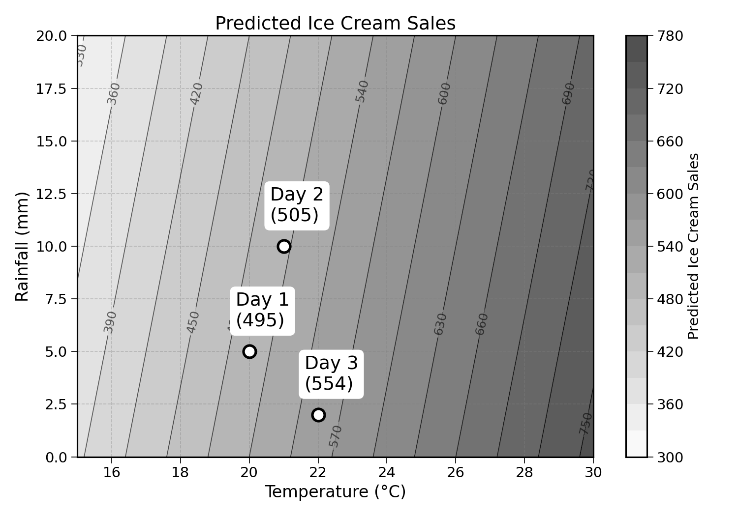
First, we can use a contour plot, using the two input features (temperature and rainfall) as axes and ice cream sales for the contour:
We could also plot the object defined by this function by using perspective to give the illusion of a third dimension:
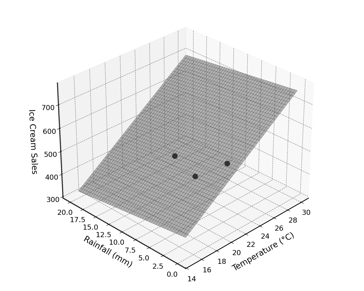
You may notice something interesting. In two dimensions, a linear regression is a single line. In three dimensions, it becomes a plane (a flat sheet of paper). In four dimensions or more (when you have 3 or more input variables), it becomes a hyperplane.
A hyperplane is not a fancy flying vehicle. It is the name of a flat surface in higher dimensions. It is very difficult for us to imagine what a flat surface would look like in 4 or 5 dimensions. We do not have to worry about this for now.
17.3 More Notation
For a more general notation of multiple linear regression with \(k\) features (\(k = 2\) above), we can use the dot notation:
\[ \hat{y} = \beta_0 + \beta_1 \times x_1 + \beta_2 \times x_2 + \cdots + \beta_k \times x_k \]
Or the sigma notation (yes, sigma strikes again):
\[ \hat{y} = \beta_0 + \sum_{j=1}^{k} \beta_j \times x_j \]
These two notations are equivalent. This is better than having to write every single coefficient, but this notation still looks cumbersome. The following chapters will explore a better way.
Exercise 17.2 Write out the sigma notation for a multiple linear regression with 4 features (\(k = 4\)). Then write the full sum.
17.4 Final Thoughts
In this chapter, we introduced multiple linear regression as a way to make predictions using more than one input feature. Using the beta (\(\beta\)) notation, any multiple linear regression can be written concisely as:
\[ \hat{y} = \beta_0 + \sum_{j=1}^{k} \beta_j \times x_j \]
But can we do even better? The following chapters will introduce more linear algebra to represent this expression in a much more elegant way.
17.5 Solutions
Solution 17.1. Exercise 17.1
Using \(\text{Ice Cream Sales} = 10 + 25 \times \text{Temperature} - 3 \times \text{Rainfall}\):
Day 1: Temperature \(= 20\), Rainfall \(= 5\)
\[ \text{Sales} = 10 + 25 \times 20 - 3 \times 5 = 10 + 500 - 15 = 495 \]
Day 2: Temperature \(= 21\), Rainfall \(= 10\)
\[ \text{Sales} = 10 + 25 \times 21 - 3 \times 10 = 10 + 525 - 30 = 505 \]
Day 3: Temperature \(= 22\), Rainfall \(= 2\)
\[ \text{Sales} = 10 + 25 \times 22 - 3 \times 2 = 10 + 550 - 6 = 554 \]
| Day | Temperature (°C) | Rainfall (mm) | Predicted Sales |
|---|---|---|---|
| 1 | 20 | 5 | 495 |
| 2 | 21 | 10 | 505 |
| 3 | 22 | 2 | 554 |
Solution 17.2. Exercise 17.2
The sigma notation with \(k = 4\) features:
\[ \hat{y} = \beta_0 + \sum_{j=1}^{4} \beta_j \times x_j \]
Expanding the sum:
\[ \hat{y} = \beta_0 + \beta_1 \times x_1 + \beta_2 \times x_2 + \beta_3 \times x_3 + \beta_4 \times x_4 \]