3 Representing Data as Points in Space
What is data? Data can be thought of as any recorded fact. In the modern world, we tend to record facts into tables. These tables are made of rows and columns.
Using the ice cream sale example, we could record historic sales and temperatures with the following table:
| Date | Temp. (°C) | Ice Creams Sold | Humidity (%) |
|---|---|---|---|
| 2025-06-01 | 22 | 150 | 45 |
| 2025-06-02 | 24 | 180 | 50 |
| 2025-06-03 | 19 | 120 | 60 |
| 2025-06-04 | 28 | 220 | 40 |
| 2025-06-05 | 30 | 250 | 35 |
| 2025-06-06 | 25 | 200 | 42 |
Just looking at the ice cream sales and temperature observations, each of these points could also be considered a point in a two-dimensional space. This may sound very abstract, but is exactly what plots are about.
As an example, on the 6th of June 2025, the temperature was 25 degrees and 200 ice creams were sold. The point “6th of June 2025” could then be represented as the coordinates (25, 200) in a two-dimensional space of temperatures × ice cream sales.
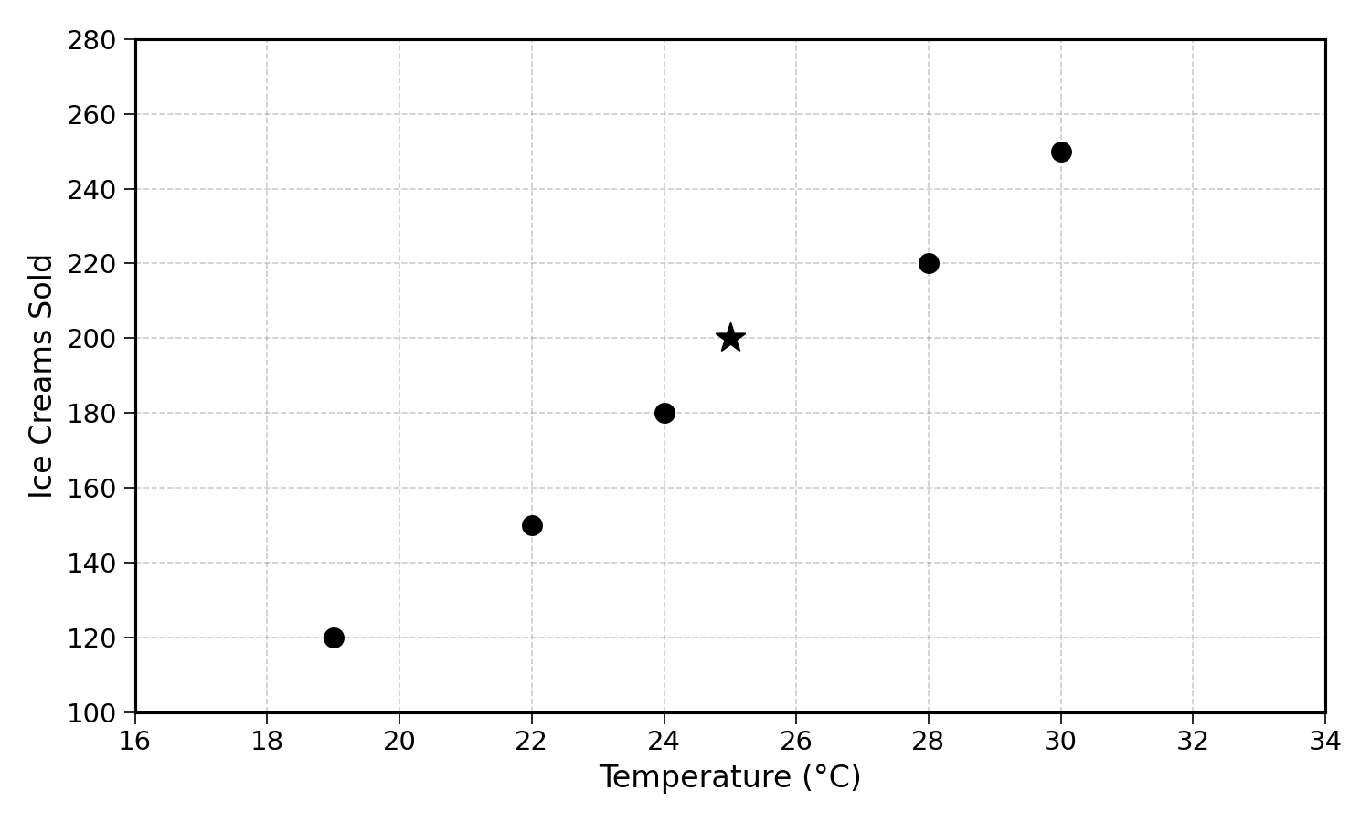
By convention, the bottom horizontal axis is called the x-axis. The vertical one is called the y-axis. The coordinates are called the x-y coordinates.
Data points can be represented in any number of dimensions. That same point of the “6th of June 2025” could have the following coordinates (25, 200, 42) in a three-dimensional space of temperatures × ice cream sales × humidity.
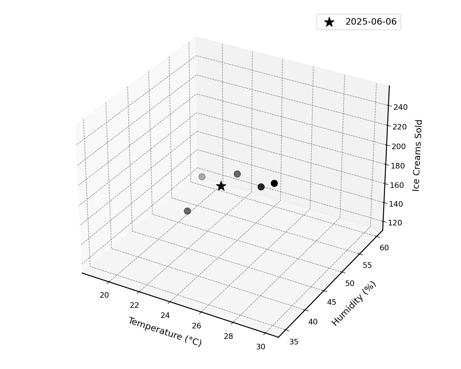
I hope that I have managed to convince you that data points can be represented and plotted as points in space.
3.1 Representing a Line in Space
Building scatter plots is fun. Can we also plot lines? In the introductory examples, we drew a line with a ruler. Can we represent this with numbers?
3.1.1 Slope
To begin with, let’s go back to ice cream sales and imagine a very small ice cream shop, that observed the following sales:
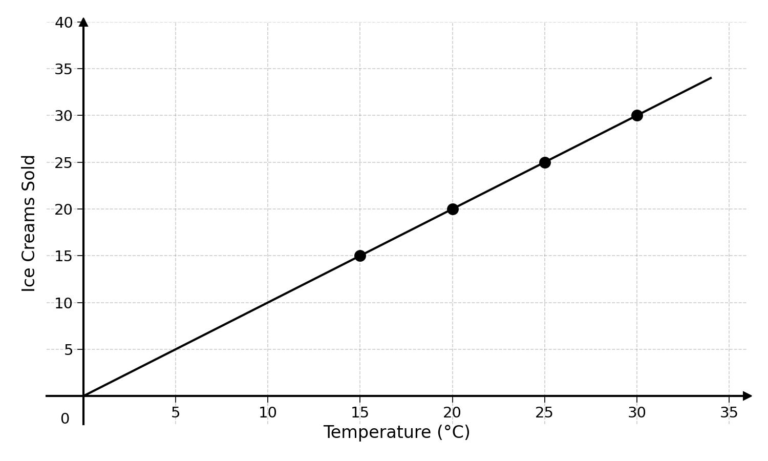
This is a highly unlikely scenario, but please, bear with me.
As you can see, all the points seem to lie on a straight line. You may also see that for each additional degree, the number of ice cream sales increases by one. We observe the following relationship:
\[ \text{Ice Cream Sales} = 1 \times \text{Degrees Celsius} \]
The 1 in this formula may seem redundant, again, bear with me.
Let’s now consider the sale of another ice cream shop:
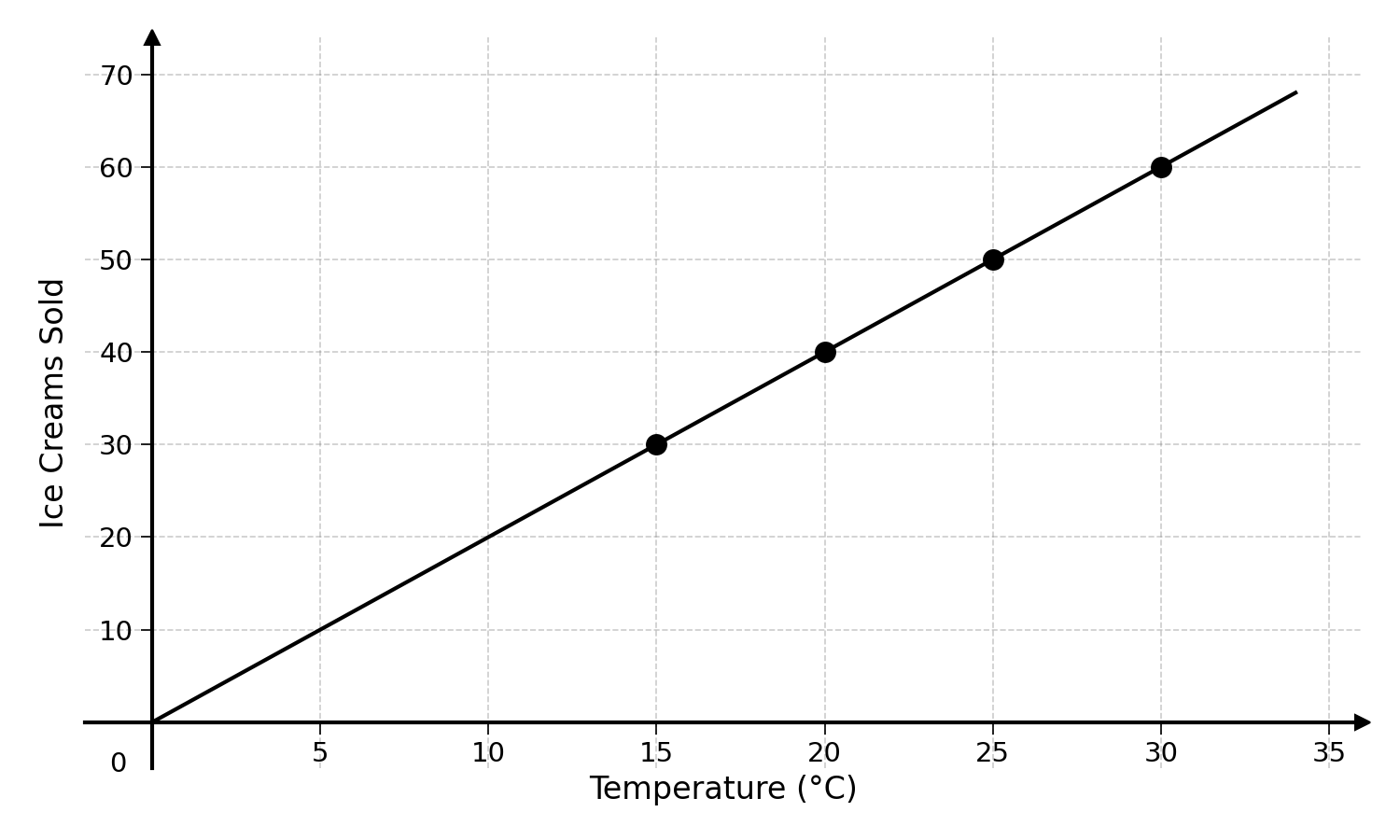
The first thought that comes to mind is: “That is a much better business”. Beyond the commercial implications, what is now the relationship between ice cream sales and temperature?
Looking at a few examples:
| Temperature (°C) | Ice Creams Sold |
|---|---|
| 20 | 40 |
| 21 | 42 |
| 22 | 44 |
| 23 | 46 |
| 24 | 48 |
| 25 | 50 |
The temperature and sales seem to obey the following relationship:
\[ \text{Ice Cream Sales} = 2 \times \text{Degrees Celsius} \]
Every additional degree Celsius brings two more ice cream sales. As you noticed, the line of the second example is steeper than in the first example.
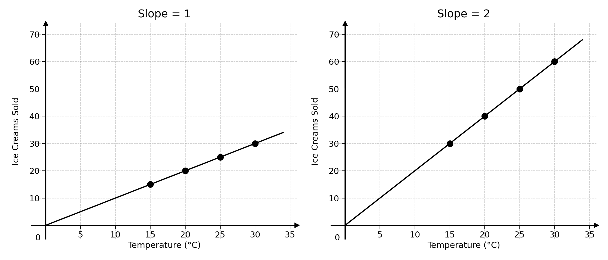
Generally, the number we multiplied the temperature by to get the sales (1 and 2 respectively) is called the slope of the line. It is its rate of increase. A higher slope will mean that ice cream sales increase faster with temperature.
3.1.2 Intercept
Now, let’s imagine that our ice cream shop has 10 customers that buy ice cream everyday, for every temperature above 0.
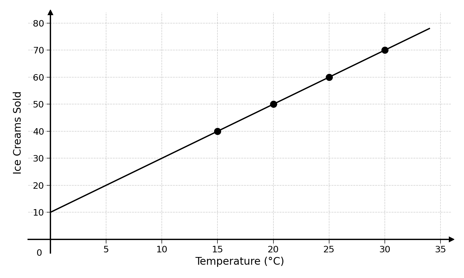
Having a loyal customer base provides some stability for such a weather-dependent business.
How would you now describe the relationship between temperature and sales?
We could use the same slope as before and just add 10, for the loyal customers who come regardless of temperature:
\[ \text{Ice Cream Sales} = 10 + 2 \times \text{Degrees Celsius} \]
This 10 is also called the intercept. Why do you think that is? Looking at the value of the line when the temperature is 0 may make this more apparent:
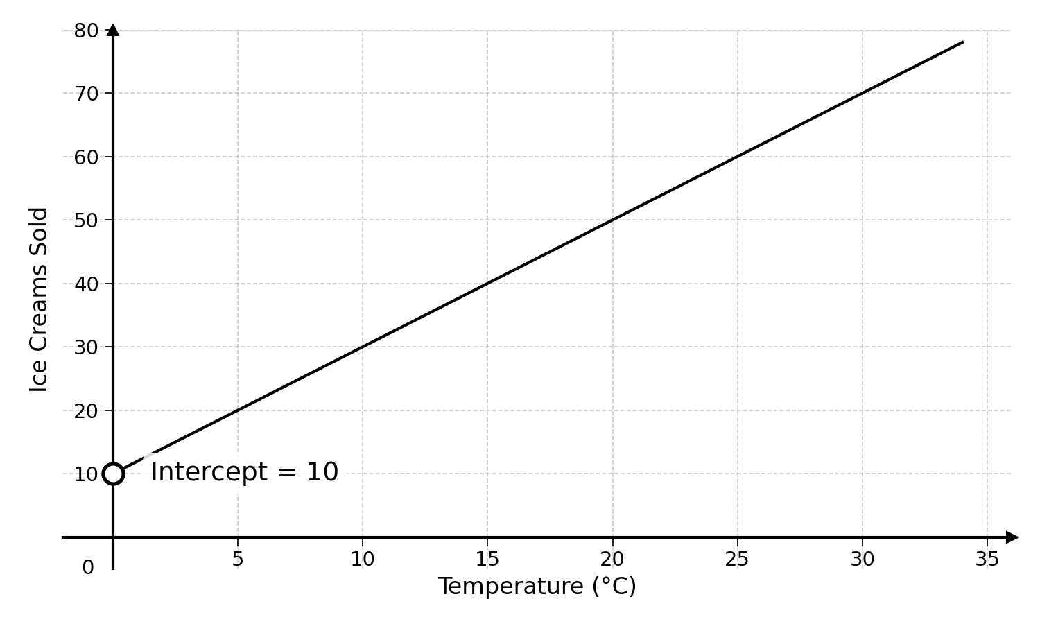
The intercept is the value of the line when it crosses the y-axis, when x is 0. Believe it or not, with the slope and the intercept, you can describe any line in a two-dimensional space.
3.2 General Formulation
Let’s move away from the ice cream sales example to a more general formulation. The line:
\[ \text{Ice Cream Sales} = 10 + 2 \times \text{Degrees Celsius} \]
Can also be written as:
\[ y = 10 + 2 \times x \]
What happened there? We moved from nice friendly words we can all relate to, to scary letters \(x\) and \(y\).
In this example, \(x\) would be the temperature in degrees and \(y\) the number of ice creams sold. In mathematics, we use letters from the end of the alphabet to represent variables. Variables are mathematical objects that can take on different values. By convention, we use letters from the end of the alphabet (e.g., \(x\), \(y\), \(z\)) to represent variables and letters from the beginning of the alphabet (e.g., \(a\), \(b\), \(c\)) to represent constants.
For example, the number of degrees Celsius could be anything from absolute zero (−273 degrees Celsius) to any positive temperature observable on earth. At the time of writing, the highest temperature ever recorded on earth was around 56 degrees Celsius (134 degrees Fahrenheit) in California in 1913.
Similarly, \(y\) could take on any value from 0 (negative sales are not expected) to the number of ice creams in stock on that day.
These variables can be manipulated like normal numbers. The expression above describes a relationship between two numbers: the number of ice cream sales and the observed temperature.
The expression \(y = 10 + 2 \times x\) simply means that for any number \(x\), \(y\) is defined by \(10 + 2 \times x\). This means that the value of \(y\) would change with the value of \(x\).
Going back to lines, any line in a two-dimensional space can be represented by two numbers, its slope and its intercept. Its slope defines how steep the line is and the intercept the value at which the line crosses the y-axis (when \(x\) is equal to 0).
3.3 Practical Exercise: Guessing the Slope and the Intercept
What is the slope and the intercept of this line?
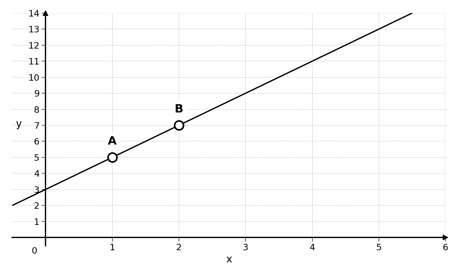
The intercept is the easiest to guess, as it is the value of the line at \(x = 0\), when it crosses the y-axis: 3. Back to the ice cream example, it is the number of loyal customers that come for any positive temperature.
The slope is the amount that \(y\) increases when \(x\) increases by one. In the ice cream example, it is the number of additional ice creams sold when the temperature increases by one degree.
To calculate this number, you can take any two points of the plot, and divide the change in \(y\) (ice creams sold) by the change in \(x\) (additional degrees).
The two points highlighted in the chart above have the following coordinates:
- A: (1, 5)
- B: (2, 7)
Between these two points, \(y\) increased by 2 and \(x\) increased by 1.
\[ \text{Slope} = \frac{\text{Increase of } y}{\text{Increase of } x} = \frac{y_B - y_A}{x_B - x_A} = \frac{7 - 5}{2 - 1} = \frac{2}{1} = 2 \]
Well done, you can now guess the slope of any line!
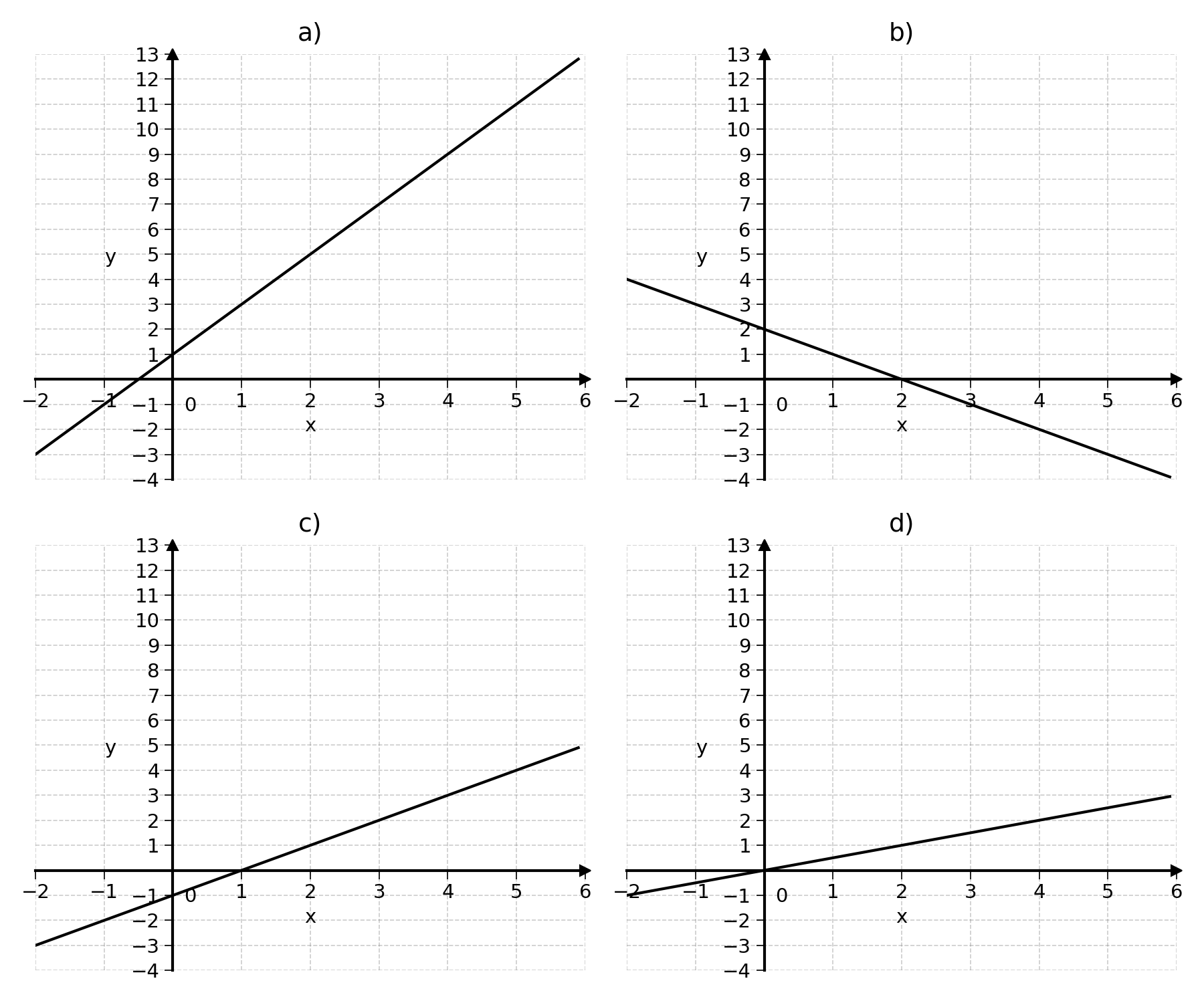
Exercise 3.1 Guess the slope and intercept of the following lines:
3.4 Final Thoughts
In this chapter we defined any line in two dimensions with two numbers: the slope and the intercept. The lines that were used in the first chapter to predict electricity production and ice cream sales were also defined by a slope and an intercept.
The main problem of linear regression is to find the optimal slope and intercept, to find the line that will provide the best estimation of the data. But this will come in due time.
The next chapter will cover functions, another foundational mathematical object to understand linear regression.
3.5 Solutions
Solution 3.1. Exercise 3.1
- Line: \(y = 1 + 2x\)
- Intercept: 1 (where the line crosses the y-axis)
- Slope: 2 (for each unit increase in \(x\), \(y\) increases by 2)
- Line: \(y = 2 - x\)
- Intercept: 2
- Slope: −1 (negative slope means the line goes down as \(x\) increases)
- Line: \(y = -1 + x\)
- Intercept: −1
- Slope: 1
- Line: \(y = \frac{1}{2}x\)
- Intercept: 0 (the line passes through the origin)
- Slope: 0.5 (for each unit increase in \(x\), \(y\) increases by 0.5)