20 Fitting a Multiple Linear Regression
Concisely representing a multiple linear regression with linear algebra is important. But it does not help us find the best-fitting coefficients given the data.
To do so, we will follow the same process as with a simple linear regression and use gradient descent to minimise the mean squared error (MSE) with regards to the vector of coefficients \(\mathbf{w}\).
20.1 Computing the MSE with linear algebra
As a quick reminder, the mean squared error (MSE) is an error metric quantifying the distance between predictions and actual data.
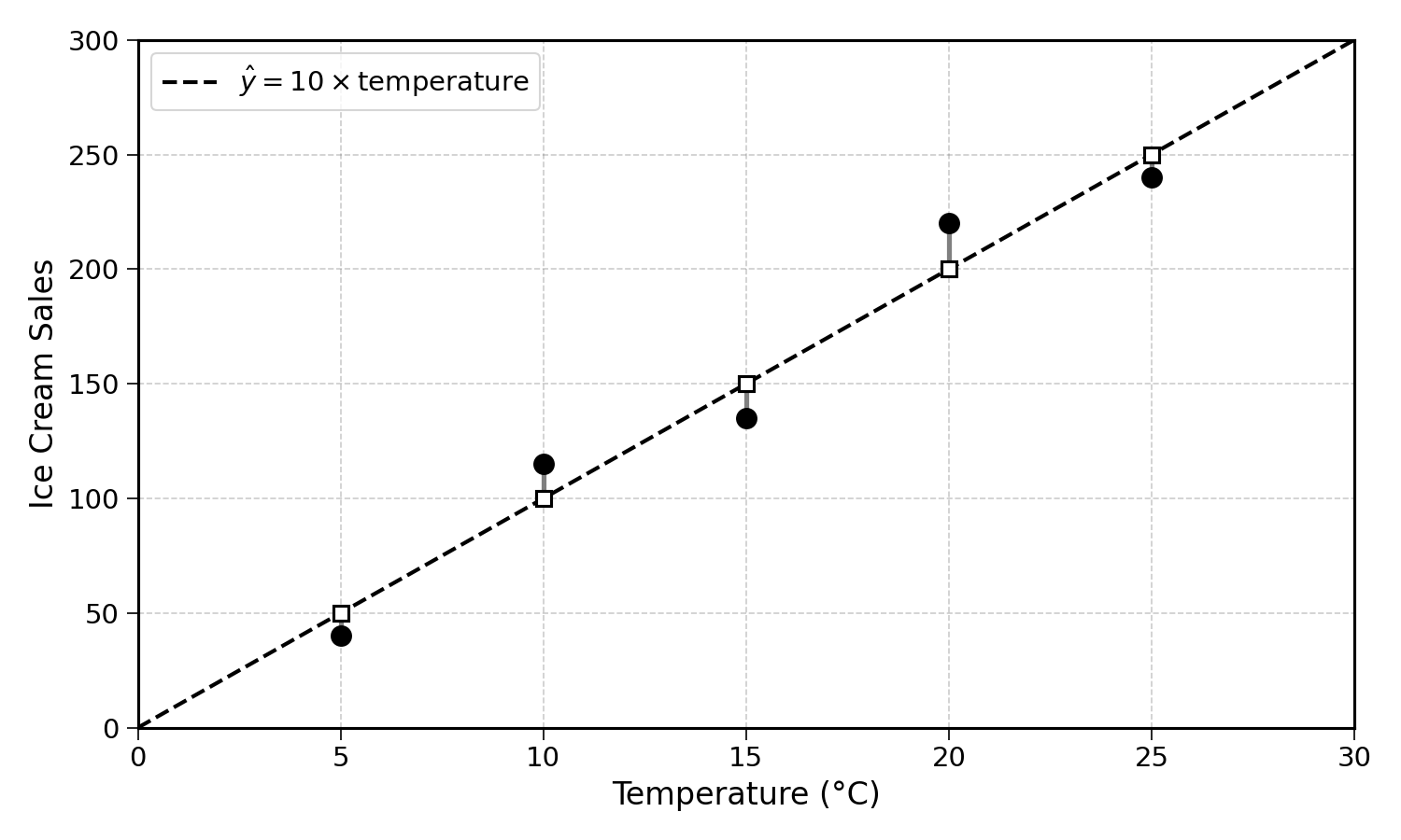
We compute the MSE by summing the squared differences between predictions and actual data:
\[ \text{MSE} = \frac{(\hat{y}_1 - y_1)^2 + (\hat{y}_2 - y_2)^2 + \cdots + (\hat{y}_n - y_n)^2}{n} = \frac{1}{n} \sum_{i=1}^{n} (\hat{y}_i - y_i)^2 \]
The above formula iterates over a list of numbers. Can we do it all in one go with vectors?
The predictions are stored in a vector \(\hat{\mathbf{y}}\). As an example, a model predicting house prices in thousands of euros could output:
\[ \hat{\mathbf{y}} = \begin{pmatrix} \hat{y}_1 \\ \hat{y}_2 \\ \hat{y}_3 \\ \hat{y}_4 \end{pmatrix} = \begin{pmatrix} 340 \\ 250 \\ 120 \\ 410 \end{pmatrix} \]
To compute the MSE, we would need another vector, noted \(\mathbf{y}\), containing the actual values.
Let’s take the following simple data as an example:
| Observation | Predicted (\(\hat{y}\)) | Actual (\(y\)) |
|---|---|---|
| 1 | 3 | 2 |
| 2 | 1 | 2 |
| 3 | 4 | 3 |
Using vector subtraction, we can obtain the vector of differences (noted \(\mathbf{e}\) for “errors”):
\[ \mathbf{e} = \hat{\mathbf{y}} - \mathbf{y} = \begin{pmatrix} 3 \\ 1 \\ 4 \end{pmatrix} - \begin{pmatrix} 2 \\ 2 \\ 3 \end{pmatrix} = \begin{pmatrix} 1 \\ -1 \\ 1 \end{pmatrix} \]
Differences are good, but we need to go one step further to calculate the MSE. We need to square all differences and calculate the average value.
From the linear algebra chapter, is there a way to get the sum of the squared values of a vector? With a dot product!
\[ \mathbf{e} \cdot \mathbf{e} = 1 \times 1 + (-1) \times (-1) + 1 \times 1 = 1 + 1 + 1 = 3 \]
Now that we have the sum of the squared differences, we just need to divide by the number of data points to get the mean squared error. Putting this all together:
\[ \text{MSE} = \frac{1}{n} (\hat{\mathbf{y}} - \mathbf{y})^T (\hat{\mathbf{y}} - \mathbf{y}) \]
Let’s use the data from the example:
\[ \hat{\mathbf{y}} - \mathbf{y} = \begin{pmatrix} 1 \\ -1 \\ 1 \end{pmatrix} \quad \text{and} \quad (\hat{\mathbf{y}} - \mathbf{y})^T = \begin{pmatrix} 1 & -1 & 1 \end{pmatrix} \]
\[ (\hat{\mathbf{y}} - \mathbf{y})^T (\hat{\mathbf{y}} - \mathbf{y}) = \begin{pmatrix} 1 & -1 & 1 \end{pmatrix} \begin{pmatrix} 1 \\ -1 \\ 1 \end{pmatrix} = 1 + 1 + 1 = 3 \]
Putting everything together:
\[ \text{MSE} = \frac{1}{3} \times 3 = 1 \]
We can now compute the MSE using vectors. This is a first step towards fitting a multiple linear regression. We now need to compute the gradient of the MSE with regards to the coefficient vector \(\mathbf{w}\).
20.2 Computing the gradient of the MSE
Like with a simple linear regression, we need the coefficient vector \(\mathbf{w}\) to appear in the MSE formula to compute the gradient:
\[ \text{MSE} = \frac{1}{n} (\hat{\mathbf{y}} - \mathbf{y})^T (\hat{\mathbf{y}} - \mathbf{y}) \]
To do so, we can substitute \(\hat{\mathbf{y}} = \mathbf{X}\mathbf{w}\) into the formula, getting:
\[ \text{MSE}(\mathbf{w}) = \frac{1}{n} (\mathbf{X}\mathbf{w} - \mathbf{y})^T (\mathbf{X}\mathbf{w} - \mathbf{y}) \]
Remember that \(\mathbf{v}^T \mathbf{v}\) is the matrix notation of a vector dot product, and that this MSE calculation is a dot product of a vector with itself.
We can then use the chain rule as we did in previous chapters, representing the MSE as a composition of functions of the coefficient vector:
\[ f(g(\mathbf{w})) \]
With:
\[ f(\mathbf{u}) = \frac{1}{n} \mathbf{u}^T \mathbf{u} \quad \text{(equivalent of } \frac{1}{n} u^2 \text{)} \]
\[ g(\mathbf{w}) = \mathbf{X}\mathbf{w} - \mathbf{y} \]
Using the chain rule, we get:
\[ \frac{d\text{MSE}}{d\mathbf{w}} = \frac{df}{dg} \times \frac{dg}{d\mathbf{w}} \]
Computing this part by part, the derivative of:
\[ f(\mathbf{u}) = \frac{1}{n} \mathbf{u}^T \mathbf{u} \quad \text{(equivalent of } \frac{1}{n} u^2 \text{)} \]
is:
\[ f'(\mathbf{u})=\frac{1}{n} \cdot 2\mathbf{u} \]
as the dot product of a vector with itself is the equivalent of squaring a scalar number. Remember that the derivative of \(x^2\) is \(2x\). We then get:
\[ \frac{df}{dg} = \frac{1}{n} \cdot 2g = \frac{2}{n}g \]
The derivative \(\frac{dg}{d\mathbf{w}}\) is slightly more complicated. The function:
\[ g(\mathbf{w}) = \mathbf{X}\mathbf{w} - \mathbf{y} \]
follows the same logic as the scalar case. The derivative of \(xw\) with respect to \(w\) is \(x\). Consider a single observation with two features \(x_1, x_2\) and two weights \(w_1, w_2\). The prediction is \(x_1 w_1 + x_2 w_2\). Its derivative with respect to \(w_1\) is \(x_1\), and with respect to \(w_2\) it is \(x_2\). The gradient is \([x_1, x_2]^T\), the features arranged as a column (just like the weights). Extending this to all observations and all weights gives \(\mathbf{X}^T\):
\[ \frac{dg}{d\mathbf{w}} = \mathbf{X}^T \]
Why this is \(\mathbf{X}^T\) and not \(\mathbf{X}\) confused me for a while when I was studying this. If you are still not convinced, the note at the end of this section should help.
Putting it all together, we get:
\[\begin{aligned} \frac{d\text{MSE}}{d\mathbf{w}} &= \frac{df}{dg} \times \frac{dg}{d\mathbf{w}} \\ &= \mathbf{X}^T \times \frac{2}{n}(\mathbf{X}\mathbf{w} - \mathbf{y}) \\ &= \frac{2}{n} \mathbf{X}^T (\mathbf{X}\mathbf{w} - \mathbf{y}) \end{aligned}\]
Putting all of this together, we get the gradient of the MSE:
\[ \nabla \text{MSE}(\mathbf{w}) = \frac{2}{n} \mathbf{X}^T (\mathbf{X}\mathbf{w} - \mathbf{y}) \]
Remember that \(\mathbf{X}\) is the feature matrix and \(\mathbf{X}\mathbf{w} - \mathbf{y}\) is the vector of errors.
With the following example, we can see that the derivative of \(g(\mathbf{w})\) has to be \(\mathbf{X}^T\) and not \(\mathbf{X}\). This is the only way we can make the multiplications work and get a final gradient of the same shape as \(\mathbf{w}\).
Let’s consider three observations and two features. The feature matrix \(\mathbf{X}\), the weight vector \(\mathbf{w}\) and the target vector \(\mathbf{y}\) are:
\[ \mathbf{X} = \begin{pmatrix} x_{11} & x_{12} \\ x_{21} & x_{22} \\ x_{31} & x_{32} \end{pmatrix} \quad \mathbf{w} = \begin{pmatrix} w_1 \\ w_2 \end{pmatrix} \quad \mathbf{y} = \begin{pmatrix} y_1 \\ y_2 \\ y_3 \end{pmatrix} \]
The predictions \(\hat{\mathbf{y}} = \mathbf{X}\mathbf{w}\) have 3 rows and 1 column, so the error vector \(\hat{\mathbf{y}} - \mathbf{y}\) also has 3 rows and 1 column, the same shape as \(\mathbf{y}\). The gradient must have the same shape as \(\mathbf{w}\), 2 rows and 1 column.
Multiplying \(\mathbf{X}\) directly by this error vector is not even a valid matrix multiplication. The number of columns of \(\mathbf{X}\), 2, does not match the number of rows of the error vector, 3.
\(\mathbf{X}^T\) is a matrix with 2 rows and 3 columns:
\[ \mathbf{X}^T = \begin{pmatrix} x_{11} & x_{21} & x_{31} \\ x_{12} & x_{22} & x_{32} \end{pmatrix} \]
Multiplying \(\mathbf{X}^T\) by the error vector gives a result with 2 rows and 1 column, exactly the shape of \(\mathbf{w}\):
\[ \mathbf{X}^T (\hat{\mathbf{y}} - \mathbf{y}) = \begin{pmatrix} x_{11} & x_{21} & x_{31} \\ x_{12} & x_{22} & x_{32} \end{pmatrix} \begin{pmatrix} \hat{y}_1 - y_1 \\ \hat{y}_2 - y_2 \\ \hat{y}_3 - y_3 \end{pmatrix} \]
Only \(\mathbf{X}^T\) produces a gradient with the same shape as \(\mathbf{w}\).
20.3 Example
Let’s compute this gradient for a concrete example. Consider the following data:
| Temperature (°C) | Ice Cream Sales |
|---|---|
| 3 | 10 |
| 4 | 11 |
| 5 | 12 |
The initial set of coefficients is:
\[ \mathbf{w}_0 = \begin{pmatrix} 2 \\ 2 \end{pmatrix} \]
With the first number the intercept and the second the slope. The feature matrix is:
\[ \mathbf{X} = \begin{pmatrix} 1 & 3 \\ 1 & 4 \\ 1 & 5 \end{pmatrix} \]
Remember that a column of \(1\)s is added on the left for the intercept in the matrix multiplication.
To get \(\mathbf{X}^T\), we swap the rows of \(\mathbf{X}\) with its columns:
\[ \mathbf{X}^T = \begin{pmatrix} 1 & 1 & 1 \\ 3 & 4 & 5 \end{pmatrix} \]
We then compute the predictions and errors:
\[ \mathbf{X}\mathbf{w}_0 = \begin{pmatrix} 1 & 3 \\ 1 & 4 \\ 1 & 5 \end{pmatrix} \begin{pmatrix} 2 \\ 2 \end{pmatrix} = \begin{pmatrix} 8 \\ 10 \\ 12 \end{pmatrix} \]
\[ \mathbf{X}\mathbf{w}_0 - \mathbf{y} = \begin{pmatrix} 8 \\ 10 \\ 12 \end{pmatrix} - \begin{pmatrix} 10 \\ 11 \\ 12 \end{pmatrix} = \begin{pmatrix} -2 \\ -1 \\ 0 \end{pmatrix} \]
Note that the starting weights mostly under-predict the actual values.
We now have all the elements to compute the gradient of the MSE for \(\mathbf{w}_0 = (2, 2)\):
\[\begin{aligned} \nabla \text{MSE}(\mathbf{w}_0) &= \frac{2}{n} \mathbf{X}^T (\mathbf{X}\mathbf{w}_0 - \mathbf{y}) \\ &= \frac{2}{3} \begin{pmatrix} 1 & 1 & 1 \\ 3 & 4 & 5 \end{pmatrix} \begin{pmatrix} -2 \\ -1 \\ 0 \end{pmatrix} \\ &= \frac{2}{3} \begin{pmatrix} 1 \times (-2) + 1 \times (-1) + 1 \times 0 \\ 3 \times (-2) + 4 \times (-1) + 5 \times 0 \end{pmatrix} \\ &= \frac{2}{3} \begin{pmatrix} -3 \\ -10 \end{pmatrix} \\ &= \begin{pmatrix} -2 \\ -6.7 \end{pmatrix} \end{aligned}\]
Both the intercept and the slope need to increase; the gradient is negative, so stepping in the opposite direction means increasing.
This makes sense considering the under-prediction mentioned above.
20.4 Using gradient descent to fit the coefficients
We now know how to calculate the mean squared error with linear algebra and compute its gradient with regards to the coefficient vector. These are all the required building blocks to minimise the MSE:
- Start with a random choice of \(\mathbf{w}_0 = (2, 2)\)
- Compute the gradient vector \(\nabla \text{MSE}(\mathbf{w})\)
- Update \(\mathbf{w}\) with the gradient update rule, using \(0.1\) as the learning rate: \[ \mathbf{w}_{t+1} = \mathbf{w}_t - \text{learning rate} \times \nabla \text{MSE}(\mathbf{w}_t) \]
- Repeat until convergence: \(\mathbf{w}_{t+1} \approx \mathbf{w}_t\)
Step 1
We have already computed the gradient of the MSE at \(\mathbf{w}_0 = (2, 2)\) above. We can substitute the values into the update equation:
\[ \mathbf{w}_1 = \begin{pmatrix} 2 \\ 2 \end{pmatrix} - 0.1 \times \begin{pmatrix} -2 \\ -6.7 \end{pmatrix} = \begin{pmatrix} 2 + 0.2 \\ 2 + 0.7 \end{pmatrix} = \begin{pmatrix} 2.2 \\ 2.7 \end{pmatrix} \]
Step 2
With \(\mathbf{w}_1 = (2.2, 2.7)\), compute predictions and errors:
\[ \mathbf{X}\mathbf{w}_1 = \begin{pmatrix} 1 & 3 \\ 1 & 4 \\ 1 & 5 \end{pmatrix} \begin{pmatrix} 2.2 \\ 2.7 \end{pmatrix} = \begin{pmatrix} 10.3 \\ 13.0 \\ 15.7 \end{pmatrix} \]
\[ \mathbf{X}\mathbf{w}_1 - \mathbf{y} = \begin{pmatrix} 10.3 \\ 13.0 \\ 15.7 \end{pmatrix} - \begin{pmatrix} 10 \\ 11 \\ 12 \end{pmatrix} = \begin{pmatrix} 0.3 \\ 2.0 \\ 3.7 \end{pmatrix} \]
\[\begin{aligned} \nabla \text{MSE}(\mathbf{w}_1) &= \frac{2}{3} \begin{pmatrix} 1 & 1 & 1 \\ 3 & 4 & 5 \end{pmatrix} \begin{pmatrix} 0.3 \\ 2.0 \\ 3.7 \end{pmatrix} \\ &= \frac{2}{3} \begin{pmatrix} 6.0 \\ 27.4 \end{pmatrix} = \begin{pmatrix} 4.0 \\ 18.3 \end{pmatrix} \end{aligned}\]
\[ \mathbf{w}_2 = \begin{pmatrix} 2.2 \\ 2.7 \end{pmatrix} - 0.1 \times \begin{pmatrix} 4.0 \\ 18.3 \end{pmatrix} = \begin{pmatrix} 1.8 \\ 0.9 \end{pmatrix} \]
Notice the oscillation: the slope jumped from \(2\) to \(2.7\) and back down to \(0.9\). This is gradient descent correcting itself, similar to what we saw in previous chapters. After many more iterations, the algorithm converges to the optimal coefficients.
Exercise 20.1 Consider the following data:
| Temperature (°C) | Ice Cream Sales |
|---|---|
| 1 | 5 |
| 2 | 7 |
| 3 | 9 |
Starting from \(\mathbf{w}_0 = (2, 2)\) with a learning rate of \(0.05\):
- Write out the feature matrix \(\mathbf{X}\) (with a column of \(1\)s) and the vector \(\mathbf{y}\).
- Compute the predictions \(\mathbf{X}\mathbf{w}_0\) and the errors \(\mathbf{X}\mathbf{w}_0 - \mathbf{y}\).
- Compute \(\nabla \text{MSE}(\mathbf{w}_0) = \frac{2}{3} \mathbf{X}^T (\mathbf{X}\mathbf{w}_0 - \mathbf{y})\).
- Update \(\mathbf{w}_1 = \mathbf{w}_0 - 0.05 \times \nabla \text{MSE}(\mathbf{w}_0)\).
- What line do you think the algorithm is converging to?
20.5 Final Thoughts
Fitting a multiple linear regression is very similar to fitting a simple linear regression. The most difficult part of this process is understanding all of its core components: functions, derivatives, linear algebra, gradient descent. But you made it, congratulations.
The key result of this chapter is the gradient formula:
\[ \nabla \text{MSE}(\mathbf{w}) = \frac{2}{n} \mathbf{X}^T (\mathbf{X}\mathbf{w} - \mathbf{y}) \]
This single expression works for any number of features and any number of observations. Whether fitting a simple regression with one slope or a model with hundreds of features, the same formula and the same algorithm apply.
20.6 Solutions
Solution 20.1. Exercise 20.1
1. The feature matrix and target vector:
\[ \mathbf{X} = \begin{pmatrix} 1 & 1 \\ 1 & 2 \\ 1 & 3 \end{pmatrix} \quad \text{and} \quad \mathbf{y} = \begin{pmatrix} 5 \\ 7 \\ 9 \end{pmatrix} \]
2. Predictions and errors:
\[ \mathbf{X}\mathbf{w}_0 = \begin{pmatrix} 1 & 1 \\ 1 & 2 \\ 1 & 3 \end{pmatrix} \begin{pmatrix} 2 \\ 2 \end{pmatrix} = \begin{pmatrix} 4 \\ 6 \\ 8 \end{pmatrix} \]
\[ \mathbf{X}\mathbf{w}_0 - \mathbf{y} = \begin{pmatrix} 4 \\ 6 \\ 8 \end{pmatrix} - \begin{pmatrix} 5 \\ 7 \\ 9 \end{pmatrix} = \begin{pmatrix} -1 \\ -1 \\ -1 \end{pmatrix} \]
3. The gradient:
\[\begin{aligned} \nabla \text{MSE}(\mathbf{w}_0) &= \frac{2}{3} \begin{pmatrix} 1 & 1 & 1 \\ 1 & 2 & 3 \end{pmatrix} \begin{pmatrix} -1 \\ -1 \\ -1 \end{pmatrix} \\ &= \frac{2}{3} \begin{pmatrix} -3 \\ -6 \end{pmatrix} = \begin{pmatrix} -2 \\ -4 \end{pmatrix} \end{aligned}\]
4. Update:
\[ \mathbf{w}_1 = \begin{pmatrix} 2 \\ 2 \end{pmatrix} - 0.05 \times \begin{pmatrix} -2 \\ -4 \end{pmatrix} = \begin{pmatrix} 2.1 \\ 2.2 \end{pmatrix} \]
5. The data follows the line \(y = 3 + 2x\), so the algorithm is converging to \(\mathbf{w} = (3, 2)\).