7 Fitting a Linear Regression
As shown in the previous chapters, different lines can provide better or worse predictions of historical data. Using the same three observations as before:
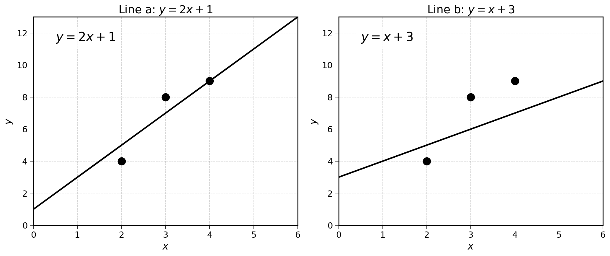
Model a seems to be much more accurate than model b. This qualitative observation can be confirmed by computing the mean squared error of both models. Model a has an MSE of 0.67, compared to an MSE of 3 for model b.
Having more accurate predictions helps us make better planning decisions. For example, a good prediction of ice cream sales tomorrow will help hire the right number of people and better manage inventory. It is in our interest to find the best regression line possible.
The process of finding the best regression line for a training dataset is referred to as fitting, training, or “finding the line of best fit”. The mean squared error (MSE) is our measure of “goodness of fit”. A low mean squared error implies that the regression line fits the data well.
How can we find this line of best fit?
7.1 Random Search
This is not an easy problem, yet, there are easy approaches. The first one would be to try many different lines, compute their MSE and pick the best one. This may sound simple, but could already give decent results.
Remembering that a line in two dimensions is defined by a slope (\(a\)) and an intercept (\(b\)):
\[ y = ax + b \]
We could try different values of \(a\) and \(b\). If you are going to stop reading here, just remember that you should not try this at home. There are stabler methods to fit a linear regression. They are the topic of the rest of this section.
Running an experiment, we could randomly pick a few different combinations of \(a\) and \(b\). Some examples are shown below:
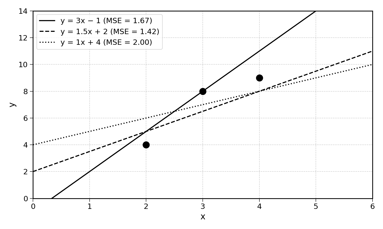
These lines will have different MSEs. Computing them:
| Line | Equation | MSE |
|---|---|---|
| 1 | \(y = 3x - 1\) | 1.67 |
| 2 | \(y = 1.5x + 2\) | 1.42 |
| 3 | \(y = x + 4\) | 2.00 |
In this case, the line of best fit seems to be \(y = 1.5x + 2\). Yet, looking at the plot, this line is not perfect. There must be a better way.
7.2 MSE and the Slope
Keeping the intercept constant at 1, we could try different slopes and examine the resulting MSE. Looking at the MSEs generated by the different slopes, a pattern starts to emerge:
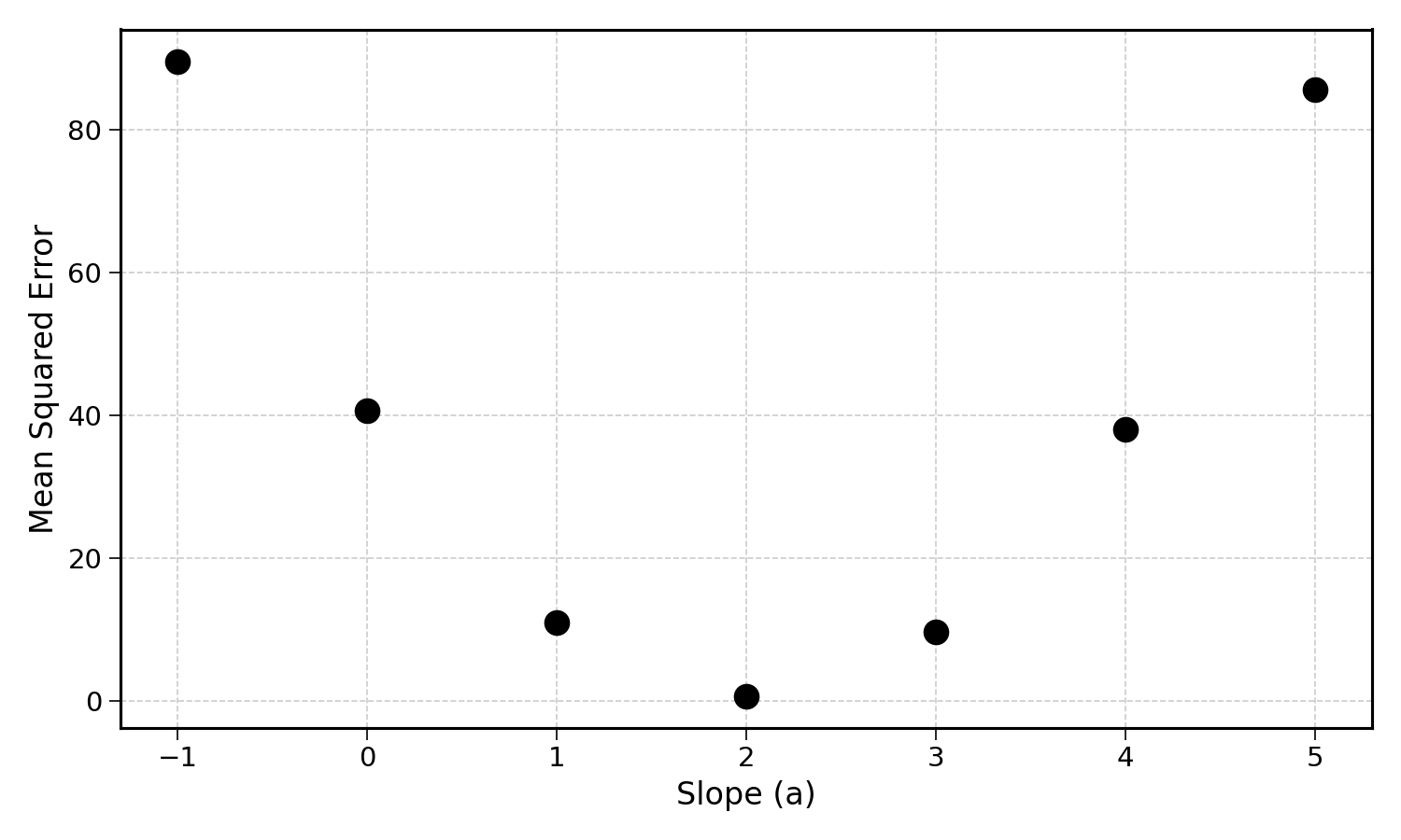
There seems to be a minimum somewhere around 2. This is interesting.
Does this apply to any dataset? We could try the same with another one. Making a guess that the intercept is 5, we try different slope values and record the resulting MSE:
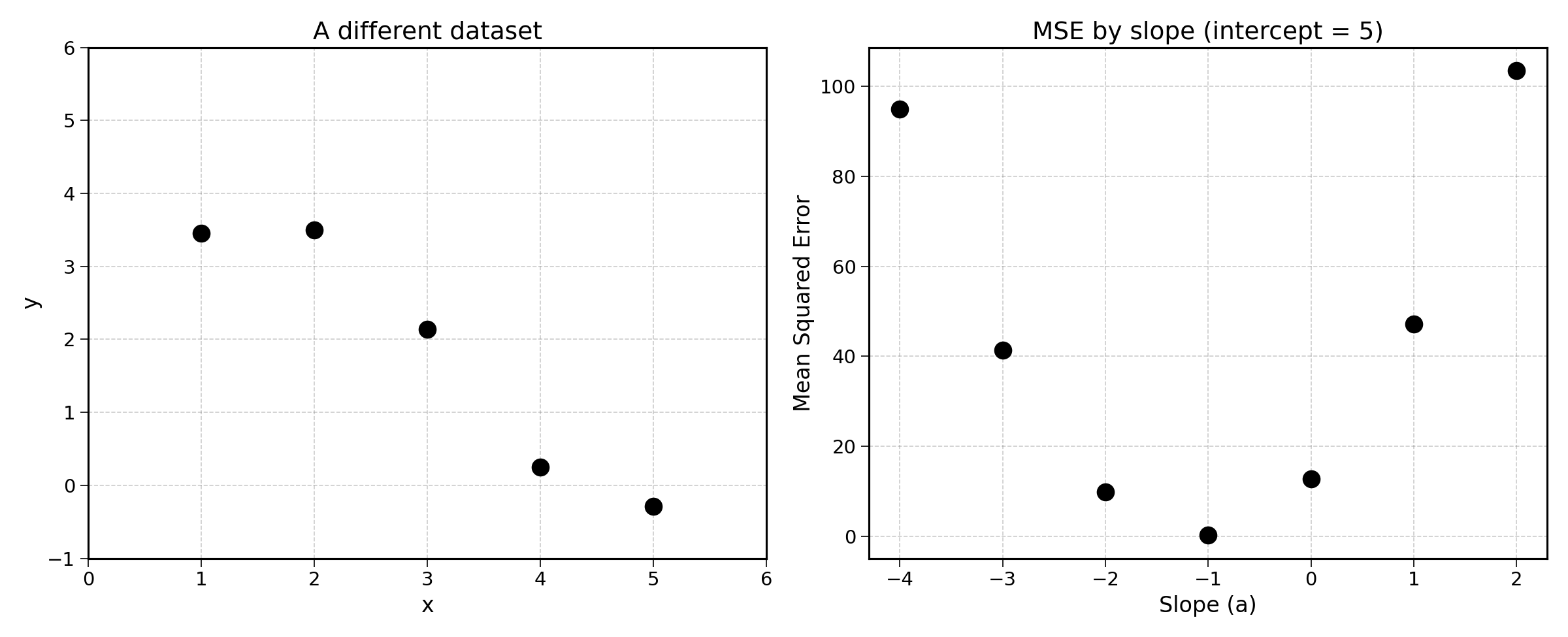
Here again, a minimum seems to exist at around \(-1\). Which looks like a good slope for the data.
We could go on like this for a while. For every new dataset, the MSE curve with regards to the slope has the same kind of behaviour. There is a minimum. Could we exploit this to find the minimum more efficiently?
7.3 Following the Curve
To find this minimum, one could just follow the curve.
For example, given this new dataset:
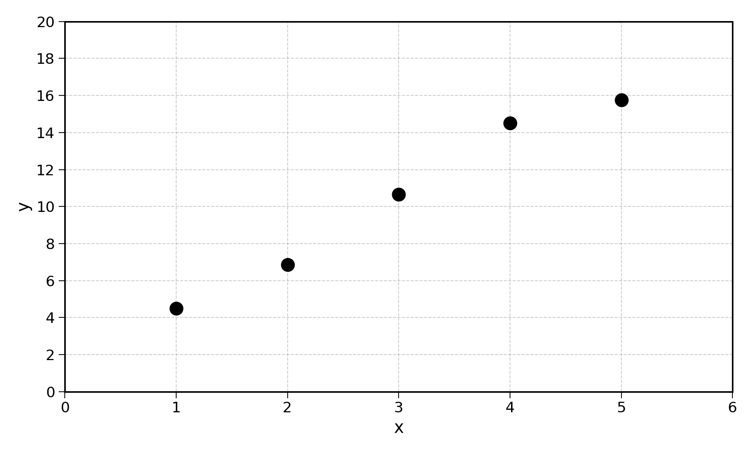
We could guess that the intercept is 1, and try 5 as our first guess for the slope. This first guess seems to over-predict quite a bit. The real slope is most likely lower. Trying progressively lower slopes (4.5, 3.75, 3.5, 3.25, 3, 2.75), the lines get closer and closer to the data. Plotting the mean squared error for each of these slope guesses alongside them, we see that the MSE goes down as the slope decreases. If the MSE and slope value have the same parabolic shape as the examples we studied before, at some point, the curve should start going back up:
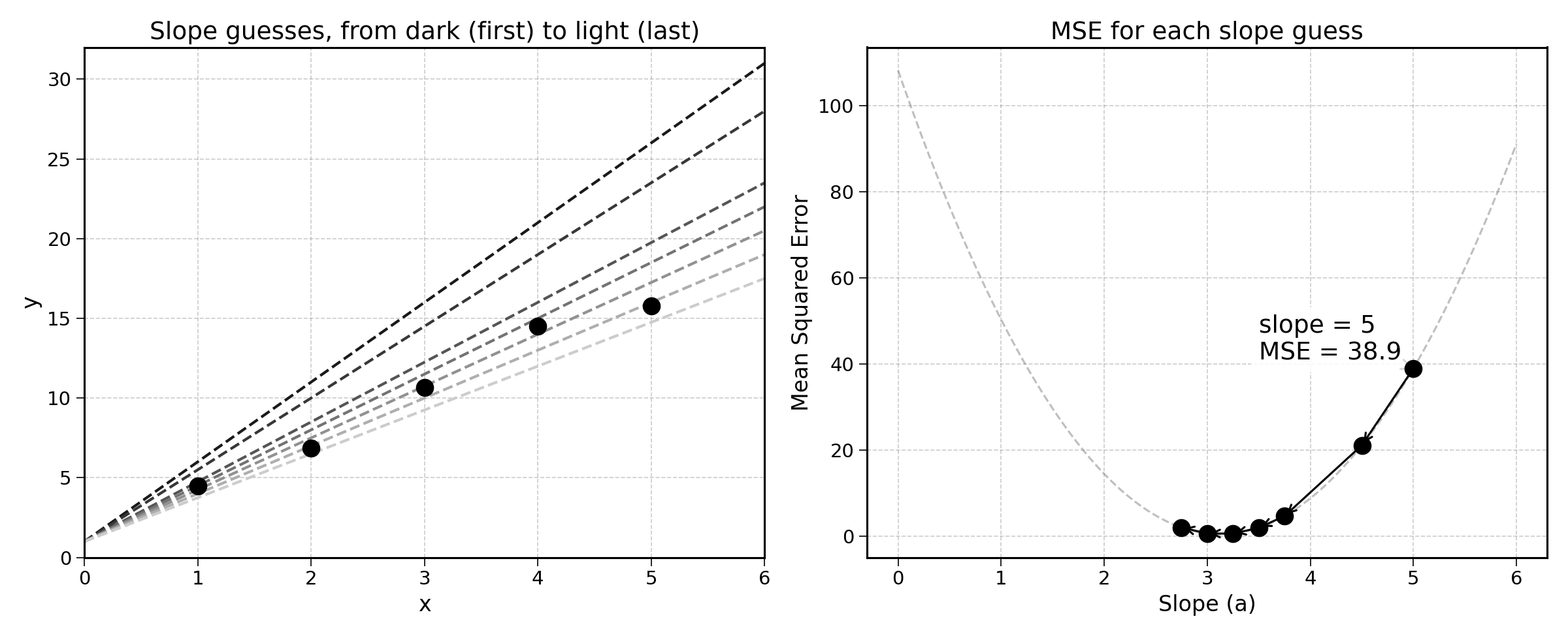
We can see a minimum at 3. Decreasing the slope from 3 to 2.75 causes an increase in prediction error. With this method, we are sure to find the slope that generates the lowest prediction error. In addition, we do not need to try dozens of random slope values. An improvement over random search.
7.4 Final Thoughts
This process of following the curve of the error still requires manual effort. Can we find the minimum of this curve in a more efficient way?
Yes! The MSE curve has a clear minimum, and there are mathematical tools that can find it efficiently. The next section of this book will introduce derivatives and gradient descent, two concepts that will allow us to find the best fitting line automatically.
The word “derivative” may bring back some high school memories. I have done my best to make them as easy as possible to understand. Even if you already know about derivatives, the following chapters may still teach you a thing or two.