12 Functions with Multiple Inputs
In the previous section, we used gradient descent to fit a linear regression with a single parameter (the slope). The problem could be framed as minimising the function \(\text{MSE}(\text{slope})\).
A regression line has both a slope and an intercept. To optimise both at the same time, we need to work with functions that take multiple inputs. We would need to minimise the function \(\text{MSE}(\text{slope}, \text{intercept})\).
So far, this book has only considered functions with single inputs, similar to:
\[ f(x) = x^2 \]
Where the input value is \(x\) and the output value \(f(x)\) is \(x^2\). Some functions can take multiple inputs. For example:
\[ f(x_1, x_2) = x_1 + x_2 \]
or:
\[ g(x_1, x_2) = x_1^2 + 2x_2 \]
Here, \(f(1, 2)\) would be equal to \(1 + 2 = 3\). So far so good.
Exercise 12.1 Compute \(g(2, 3)\) and \(g(1, 5)\) for the function \(g(x_1, x_2) = x_1^2 + 2x_2\).
12.1 Plotting Functions with Multiple Inputs
These functions with multiple inputs are more difficult to plot than the single input functions, as there are now three dimensions we are interested in: \(x_1\), \(x_2\), and \(f(x_1, x_2)\), the output value. As this book is printed on flat pages, plotting a third dimension is not trivial. There are several tricks one could use.
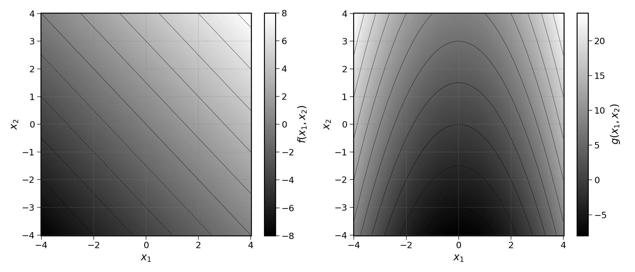
One of them is a shade plot, in which shading represents the output value of the function and the two axes represent the two inputs. The colour bar on the right shows which shade corresponds to which output value. Plotting \(f\) and \(g\), we get the following shade plots:
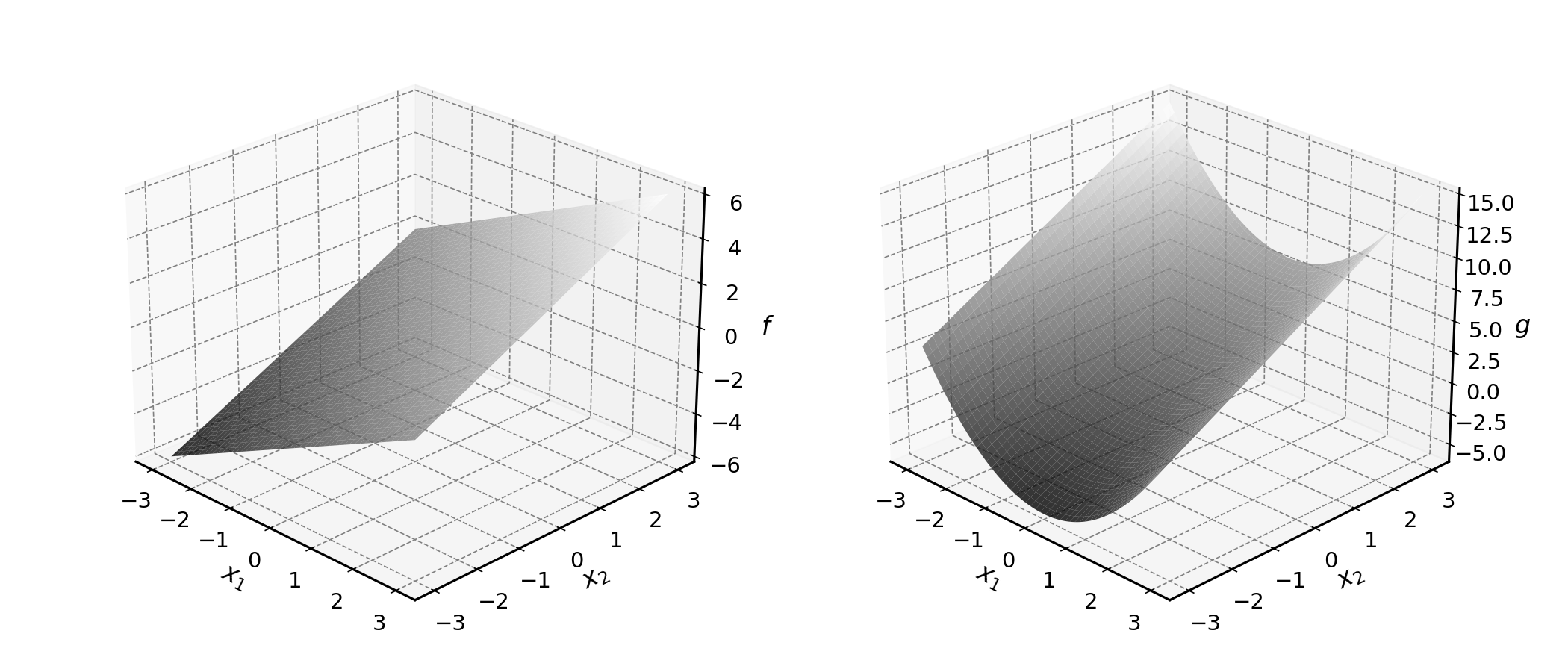
A more sophisticated method involves using perspective to give the illusion of depth. This is exactly what Italian Renaissance painters used to depict three-dimensional forms on a two-dimensional canvas. Plotting \(f\) and \(g\) with perspective, we get the following surface plots:
12.2 Plotting the MSE
Using the ice cream data from the previous chapter, the MSE of the linear regression can be expressed as a function of two parameters, the slope and the intercept.
The MSE can be plotted as a two-dimensional shade plot:
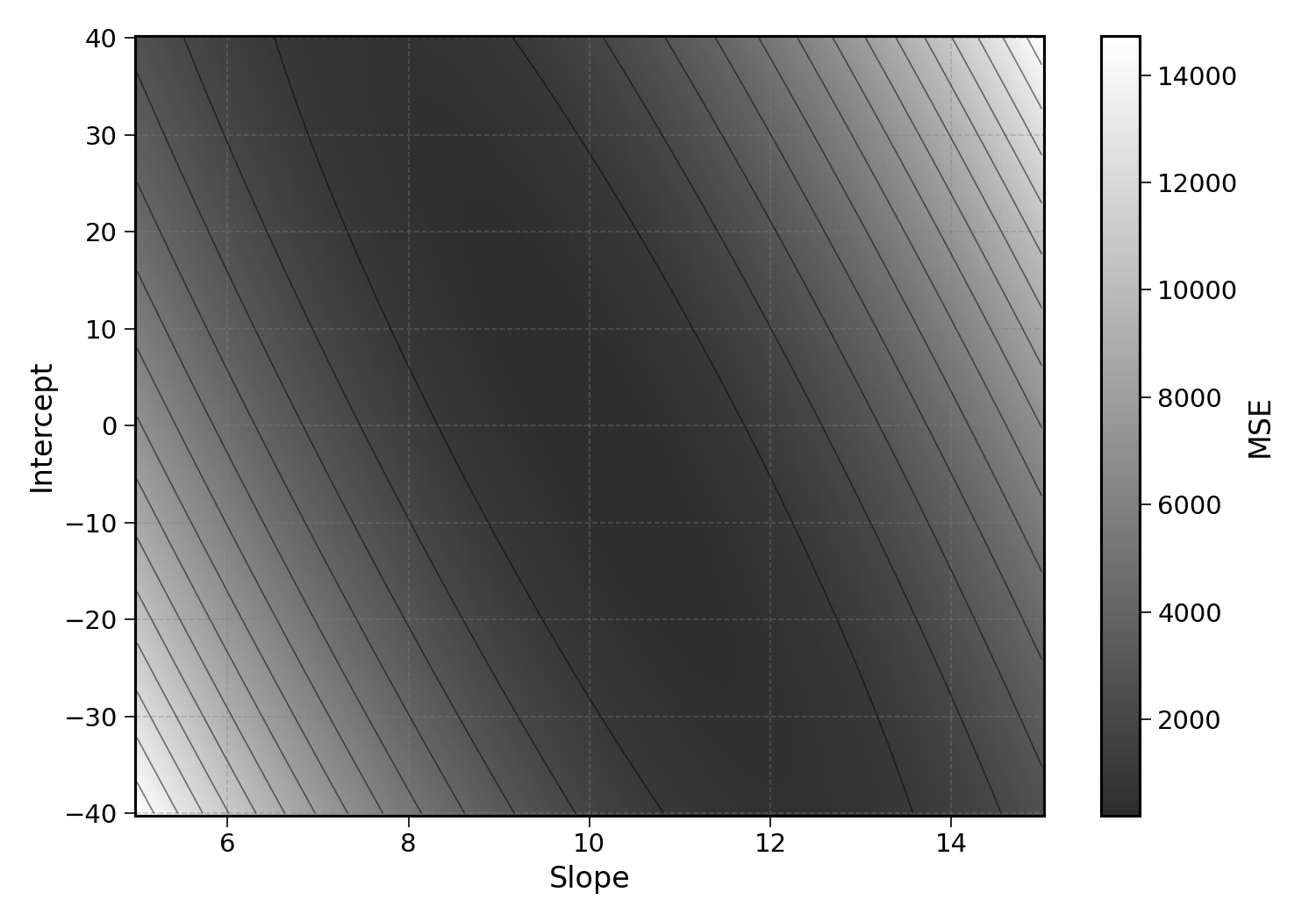
The darker area in the centre of the plot corresponds to the lowest MSE values. This is where the optimal slope and intercept lie. As we had calculated, the optimal slope and intercept are 10 and 0 respectively.
The same function can also be plotted as a three-dimensional surface:
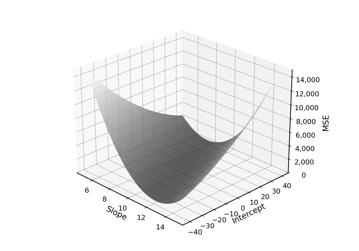
The goal of gradient descent is to find the bottom of this bowl, the combination of slope and intercept that minimises the MSE.
12.3 Final Thoughts
This chapter only covered functions with two inputs, as they are the most convenient to plot on a two-dimensional page. But there can be functions with many more inputs, like:
\[ f(x_1, x_2, x_3) = (x_1 + x_2) \times x_3 \]
or even:
\[ g(x_1, x_2, \ldots, x_n) = \sum_{i=1}^{n} x_i \]
As the number of inputs grows, the notation above will become more cumbersome. It is time to introduce a way to handle collections of numbers: vectors.
12.4 Solutions
Solution 12.1. Exercise 12.1
\[ g(2, 3) = 2^2 + 2 \times 3 = 4 + 6 = 10 \]
\[ g(1, 5) = 1^2 + 2 \times 5 = 1 + 10 = 11 \]