14 Gradient Vector
14.1 Change in Higher Dimensions
In the first part of this book, we introduced derivatives. Derivatives can be considered as the rate of change and the slope of the tangent line at a single point. Using derivatives, we can leverage gradient descent to minimise a function, by “following the derivative”.
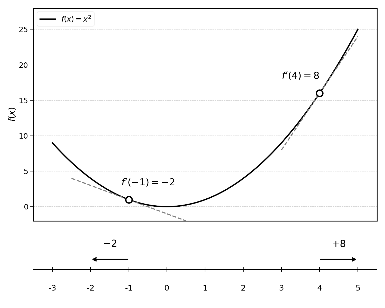
But did you wonder why gradient descent is called “gradient” descent and not “derivative” descent?
This is because a gradient is the extension of derivatives to functions with multiple inputs. If this sounds too abstract now, do not panic. This chapter will make it more concrete.
Let’s consider the function:
\[ g(x) = x^2 \]
The derivative of this function is:
\[ g'(x) = 2x \]
Now, let’s move to a function with multiple inputs:
\[ f(x_1, x_2) = x_1^2 + x_2 \]
There, we have two variables: \(x_1\) and \(x_2\). The function does not only move along a single variable \(x\). We can represent \(f(x_1, x_2)\) as a surface:
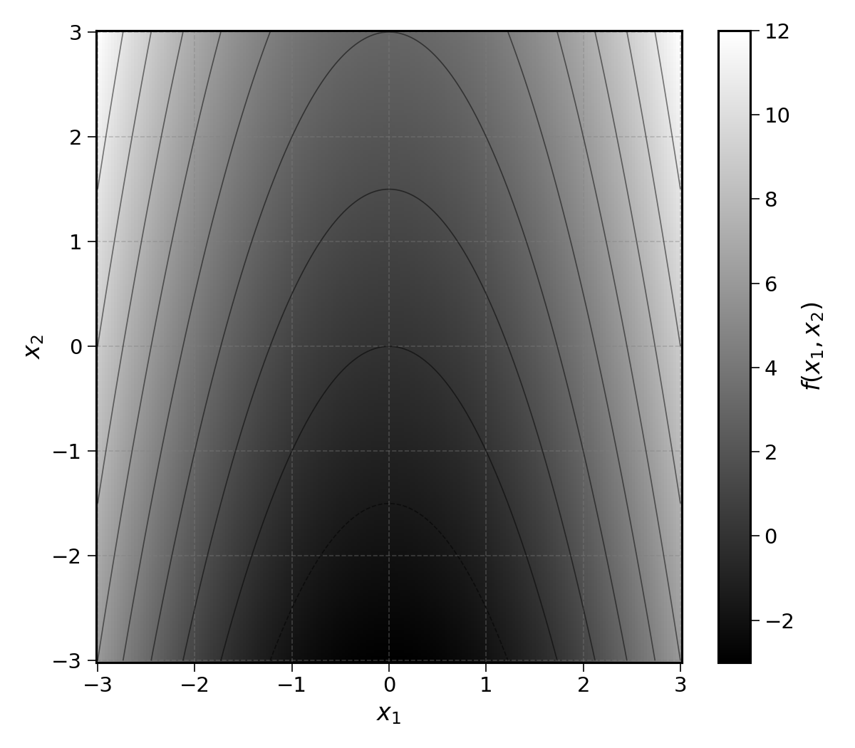
Unlike the function \(g(x)\), in which the input could only move left or right along the number line:
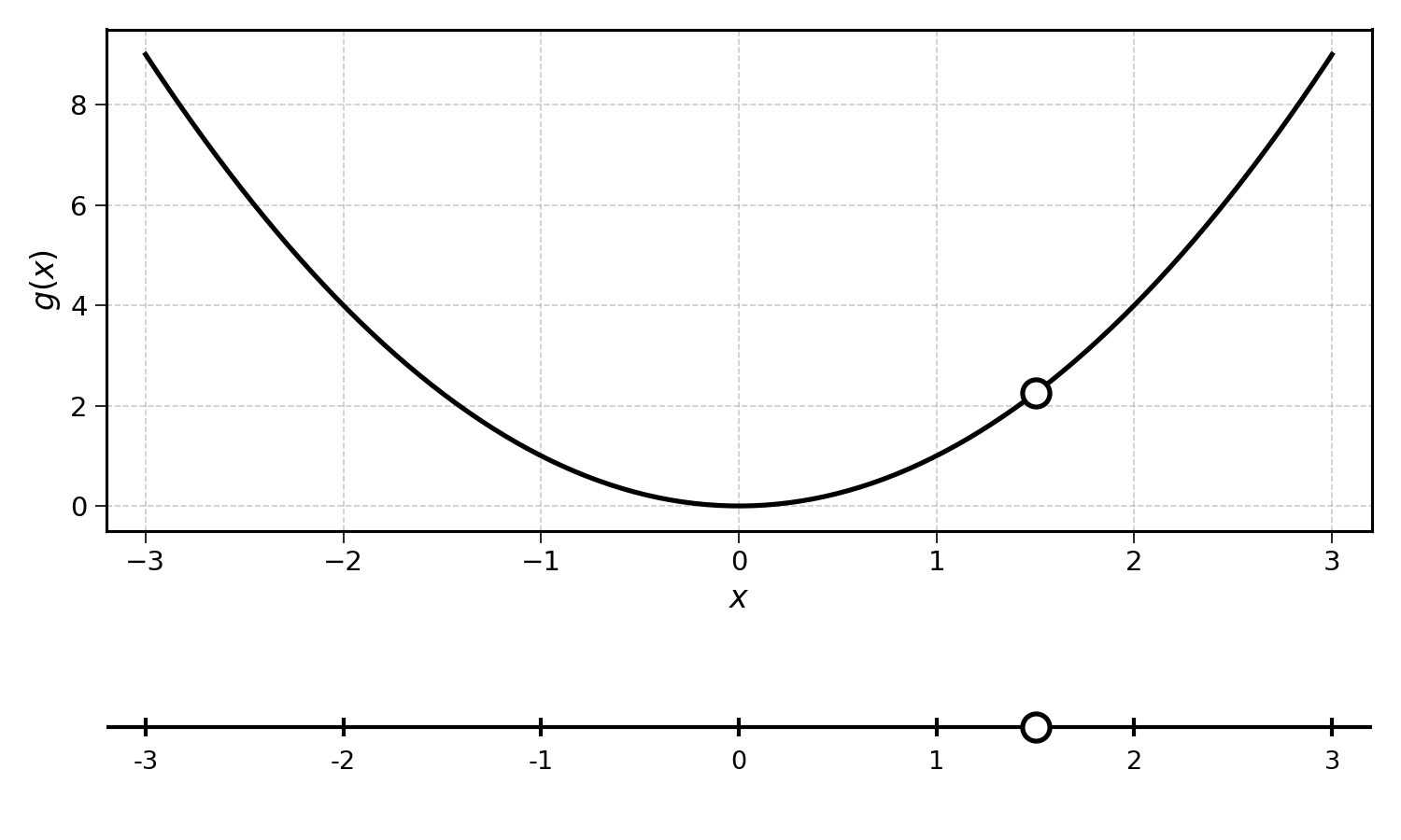
Points on the surface \(f(x_1, x_2)\) can move in many directions across a two-dimensional space:
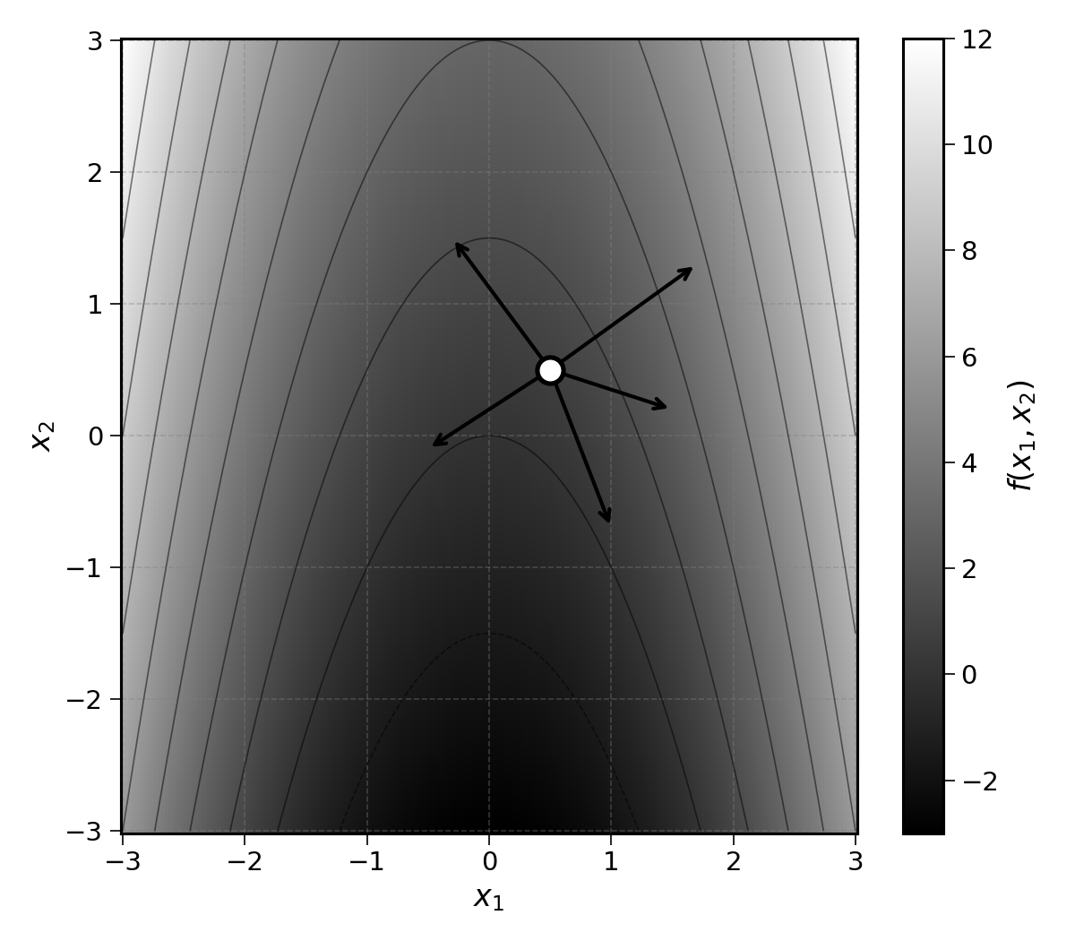
For that same reason, a function with two inputs cannot have a single tangent line, or a rate of change expressed by a single number.
Instead, the derivative of a function with multiple inputs is a vector of partial derivatives, also called the gradient vector.
14.2 The Gradient Vector
Let’s start with a concrete example:
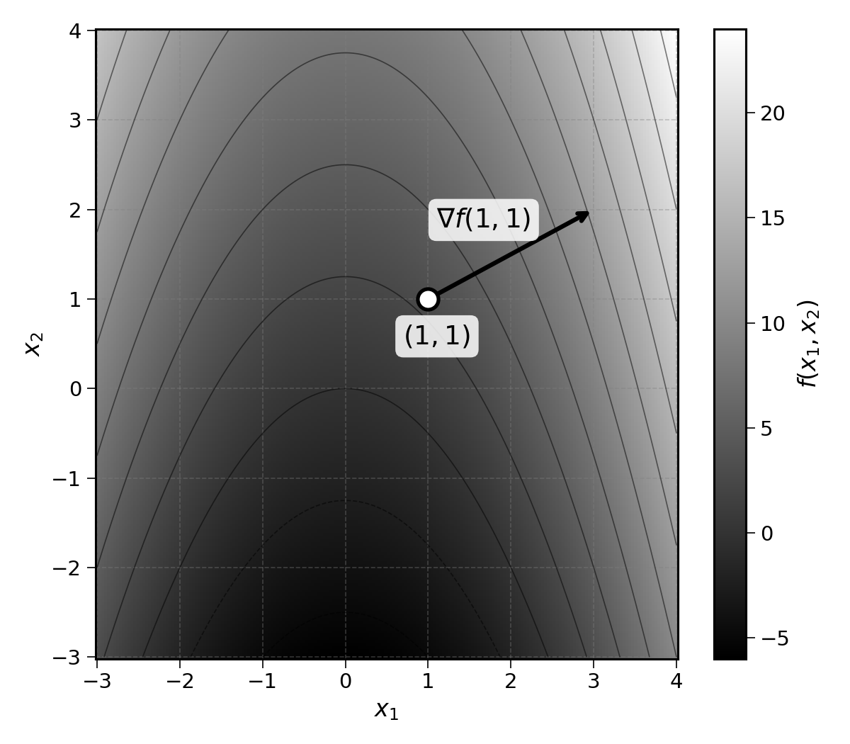
The arrow on the chart is the gradient vector; the derivative of the function \(f\) at point \((1, 1)\). This is exactly where gradient descent takes its name from.
Just like the derivative, the gradient vector points to the direction of steepest ascent.
The gradient vector has its own notation:
\[ \nabla f(x_1, x_2) = \left( \frac{\partial f}{\partial x_1}, \frac{\partial f}{\partial x_2} \right) \]
This can be broken down piece by piece. The gradient vector is nothing more than the vector of partial derivatives of a function.
14.2.1 Partial Derivatives
Imagine you are given the expression:
\[ y = a + b + 2x - 1 \]
And you want to understand how \(y\) changes with respect to the variable \(x\). In other words, you want to know \(\frac{dy}{dx}\).
To do so, you should treat all other variables as constant, and only differentiate the terms that are dependent on \(x\).
You would get:
\[ \frac{dy}{dx} = 2 \]
Every time \(x\) increases by 1, \(y\) would increase by 2.
Putting this into the language of functions: the partial derivative of a function with regards to a variable \(x\) treats all other variables as constants.
We can visualise this idea. Looking at \(f(x_1, x_2) = x_1^2 + 2x_2\), we can plot the function holding one variable constant:
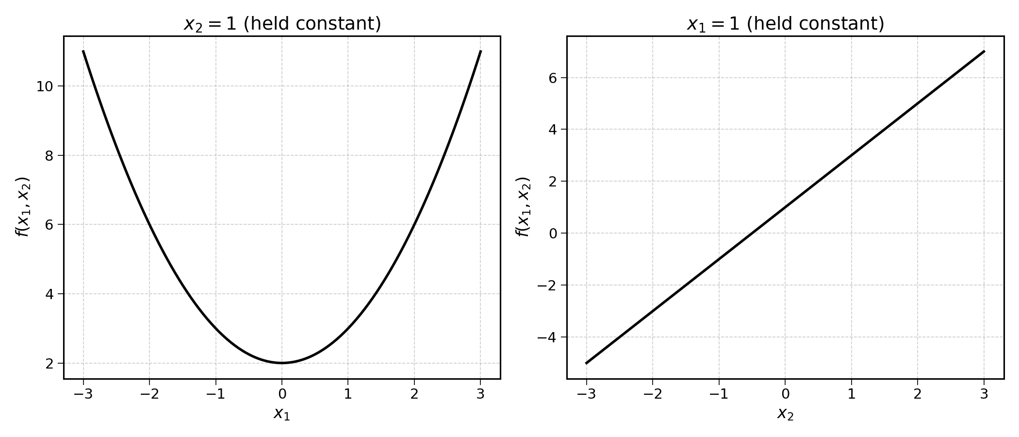
On the left, \(x_2\) is held constant at 1. The resulting curve \(f(x_1) = x_1^2 + 2\) is a parabola, just like the single-variable functions from earlier chapters. On the right, \(x_1\) is held constant at 1, and \(f(x_2) = 1 + 2x_2\) is a straight line with slope 2.
The partial derivative of a function with regards to a variable is just the derivative of the resulting single-variable function. Instead of the \(d\) used for single-variable derivatives, partial derivatives use the symbol \(\partial\), a stylised d, as a reminder that other variables are being held constant. For example, the partial derivative of:
\[ f(x_1, x_2) = x_1^2 + 2x_2 \]
with regards to \(x_1\) is:
\[ \frac{\partial f}{\partial x_1} = 2x_1 \]
As the term \(2x_2\) is treated as a constant.
Exercise 14.1 Show that the partial derivative of \(f(x_1, x_2) = x_1^2 + 2x_2\) with regards to \(x_2\) is \(2\).
The gradient vector of \(f(x_1, x_2) = x_1^2 + 2x_2\) would then be:
\[ \nabla f(x_1, x_2) = \left( \frac{\partial f}{\partial x_1}, \frac{\partial f}{\partial x_2} \right) = (2x_1, 2) \]
Just like derivatives, this gradient is the direction of steepest ascent. Using gradient information, we will be able to minimise or maximise functions with multiple inputs.
Exercise 14.2 Compute the gradient vector \(\nabla f(x_1, x_2)\) for the function \(f(x_1, x_2) = 3x_1^2 + 4x_1 x_2 + x_2^2\). Then evaluate the gradient at the point \((1, 2)\).
14.3 Final Thoughts
Functions can take more than one input. In those cases, derivatives become gradient vectors, ordered lists of partial derivatives that point in the direction of steepest ascent.
By following the direction of steepest ascent or its opposite, we can optimise these functions with multiple inputs. This is what we will need to fit both the slope and the intercept of a linear regression.
14.4 Solutions
Solution 14.1. Exercise 14.1
Taking the partial derivative of \(f(x_1, x_2) = x_1^2 + 2x_2\) with regards to \(x_2\):
The term \(x_1^2\) is treated as a constant (its derivative with regards to \(x_2\) is \(0\)).
The derivative of \(2x_2\) with regards to \(x_2\) is \(2\).
\[ \frac{\partial f}{\partial x_2} = 0 + 2 = 2 \]
Solution 14.2. Exercise 14.2
The partial derivative with regards to \(x_1\) (treating \(x_2\) as a constant):
\[ \frac{\partial f}{\partial x_1} = 6x_1 + 4x_2 \]
The partial derivative with regards to \(x_2\) (treating \(x_1\) as a constant):
\[ \frac{\partial f}{\partial x_2} = 4x_1 + 2x_2 \]
The gradient vector is:
\[ \nabla f(x_1, x_2) = (6x_1 + 4x_2, \; 4x_1 + 2x_2) \]
Evaluating at the point \((1, 2)\):
\[ \nabla f(1, 2) = (6 \times 1 + 4 \times 2, \; 4 \times 1 + 2 \times 2) = (14, \; 8) \]