16 Fitting the Slope and Intercept
We now have all the elements needed to fit both the slope and the intercept of a linear regression at the same time. As a reminder, we have covered:
- Derivatives: measure the rate of change of a function at a single point
- Partial derivatives: measure the rate of change for a single variable, treating others as constants
- Vectors: ordered lists of numbers
- Gradients: generalisation of derivatives for functions with multiple inputs
- Gradient descent: find the minimum of a function using gradient information
This chapter will put everything together to minimise the mean squared error of a linear regression by optimising both its slope and intercept for the following example data:
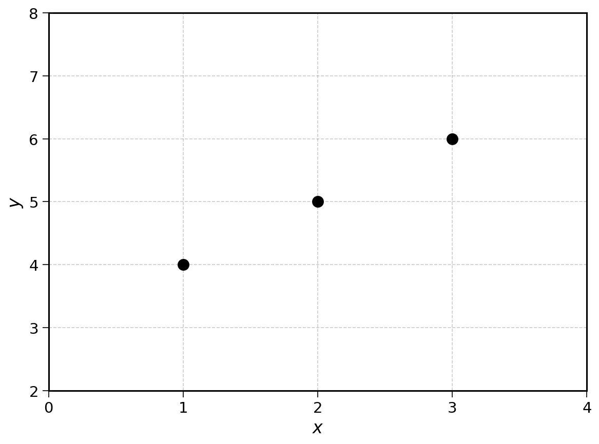
As a reminder, we represent a linear regression as:
\[ \hat{y} = \text{intercept} + \text{slope} \times x \]
and the mean squared error as:
\[ \text{MSE} = \frac{1}{n} \sum_{i=1}^{n} (\hat{y}_i - y_i)^2 \]
To minimise this function with gradient descent, we need to compute the gradient vector of the MSE. We do so using the partial derivatives with regards to both the slope and the intercept:
\[ \nabla \text{MSE} = \left( \frac{\partial \text{MSE}}{\partial \text{slope}}, \; \frac{\partial \text{MSE}}{\partial \text{intercept}} \right) \]
Let’s compute them one by one.
16.1 Partial Derivative of the MSE with Regards to the Slope
We already computed the partial derivative of the MSE with regards to the slope in a previous chapter.
After substituting \(\hat{y}_i = \text{slope} \times x_i + \text{intercept}\), the MSE can be written as:
\[ \text{MSE}(\text{slope}, \text{intercept}) = \frac{1}{n} \sum_{i=1}^{n} (\text{slope} \times x_i + \text{intercept} - y_i)^2 \]
We get the following gradient by applying the chain rule: \[\begin{aligned} \frac{\partial \text{MSE}}{\partial \text{slope}} &= \frac{1}{n} \sum_{i=1}^{n} \frac{df}{dg} \times \frac{dg}{d\text{slope}} \\ &= \frac{1}{n} \sum_{i=1}^{n} 2g \times x_i \\ &= \frac{1}{n} \sum_{i=1}^{n} 2(\text{slope} \times x_i + \text{intercept} - y_i) \times x_i \\ &= \frac{1}{n} \sum_{i=1}^{n} 2(\hat{y}_i - y_i) \times x_i \end{aligned}\]
We have the partial derivative of the MSE with regards to the slope. You may notice that it is the same as the gradient used for a linear regression with only a slope parameter in the earlier chapter. Now, let’s shift our attention to the intercept.
16.2 Partial Derivative of the MSE with Regards to the Intercept
The idea is very much the same as finding the partial derivative with regards to the slope. It also uses the chain rule. We write the inside of the summation:
\[ (\text{slope} \times x_i + \text{intercept} - y_i)^2 \]
As a composition of functions of the form \(f(g(\text{intercept}))\). Notice that the variable of interest is now the intercept.
\[ f(u) = u^2 \]
\[ g(\text{intercept}) = \text{slope} \times x_i + \text{intercept} - y_i \]
Using the chain rule:
\[ \frac{\partial \text{MSE}}{\partial \text{intercept}} = \frac{1}{n} \sum_{i=1}^{n} \frac{df}{dg} \times \frac{dg}{d\text{intercept}} \]
In the last section, we had already calculated \(\frac{df}{dg}\):
\[ \frac{df}{dg} = 2g \]
We can also compute \(\frac{dg}{d\text{intercept}}\):
\[ \frac{dg}{d\text{intercept}} = 1 \]
Why is that the case? When the intercept increases by a small amount, the function \(g(\text{intercept})\) increases by exactly the same amount.
Putting this together:
\[\begin{aligned} \frac{\partial \text{MSE}}{\partial \text{intercept}} &= \frac{1}{n} \sum_{i=1}^{n} \frac{df}{dg} \times \frac{dg}{d\text{intercept}} \\ &= \frac{1}{n} \sum_{i=1}^{n} 2g \times 1 \\ &= \frac{1}{n} \sum_{i=1}^{n} 2(\text{slope} \times x_i + \text{intercept} - y_i) \\ &= \frac{1}{n} \sum_{i=1}^{n} 2(\hat{y}_i - y_i) \end{aligned}\]
We now have both partial derivatives. This is enough for our gradient vector!
16.3 Gradient Descent of the MSE
The gradient vector of the MSE with regards to the slope and intercept is:
\[ \nabla \text{MSE}(\text{slope}, \text{intercept}) = \left( \frac{1}{n} \sum_{i=1}^{n} 2(\hat{y}_i - y_i) x_i, \;\; \frac{1}{n} \sum_{i=1}^{n} 2(\hat{y}_i - y_i) \right) \]
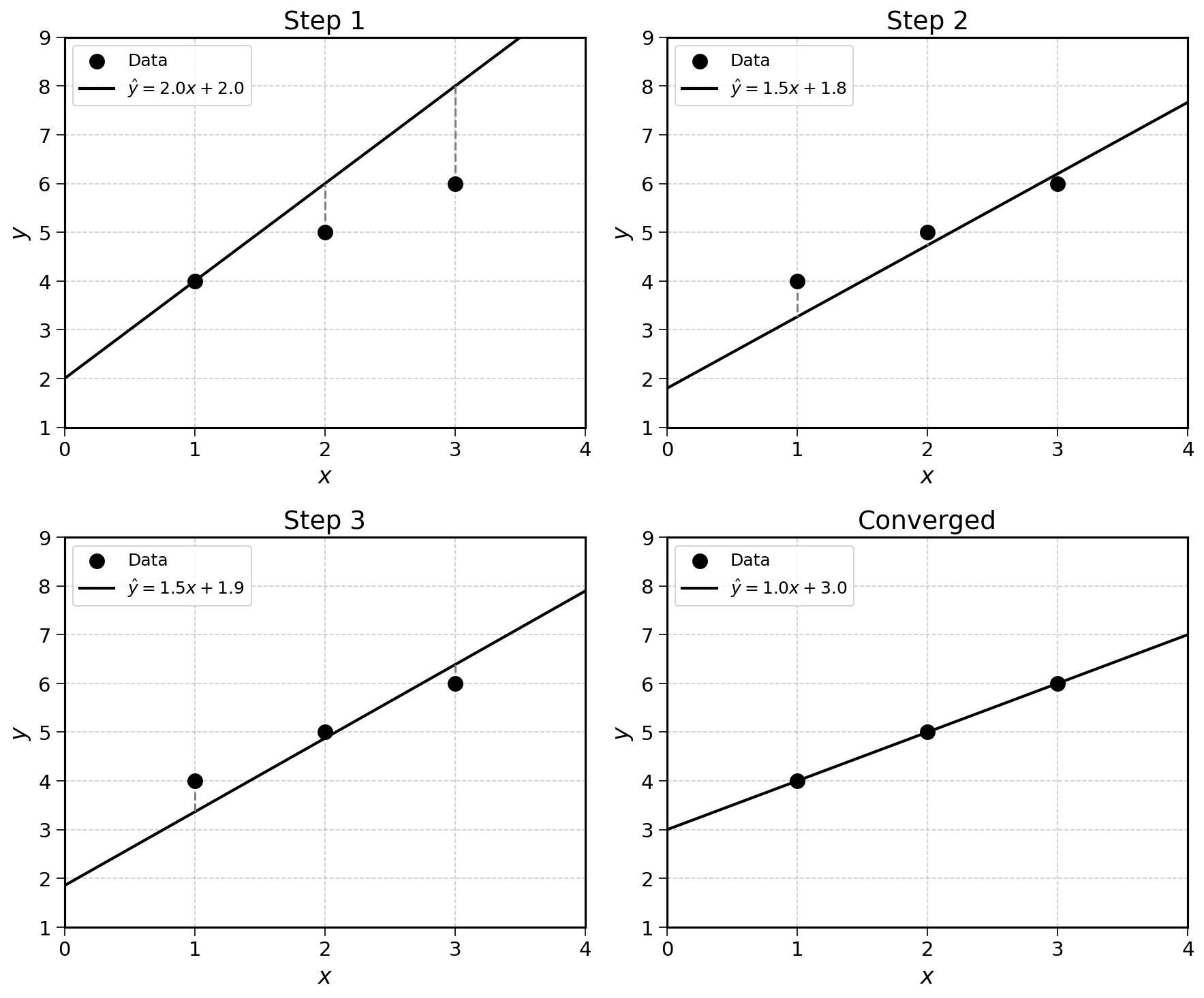
Using this vector, we can run the gradient descent algorithm to find the line of best fit. Let’s apply this to a simple example with three data points:
By visual inspection, these points seem to follow the line \(y = x + 3\). Let’s see if gradient descent can find this line.
We will note the combination of parameters as a weights vector \(\mathbf{w} = (\text{slope}, \text{intercept})\). The gradient descent steps are:
- Start with a random guess: \(\mathbf{w}_0 = (2, 2)\)
- Compute the gradient vector \(\nabla \text{MSE}(\mathbf{w})\)
- Update: \(\mathbf{w}_{t+1} = \mathbf{w}_t - \text{learning rate} \times \nabla \text{MSE}(\mathbf{w}_t)\)
- Repeat until \(\mathbf{w}_{t+1} \approx \mathbf{w}_t\)
Step 1
Start with \(\mathbf{w}_0 = (\text{slope} = 2, \text{intercept} = 2)\). The predicted values are \(\hat{y}_i = 2x_i + 2\):
| \(x_i\) | \(y_i\) | \(\hat{y}_i = 2x_i + 2\) | \(\hat{y}_i - y_i\) |
|---|---|---|---|
| 1 | 4 | 4 | 0 |
| 2 | 5 | 6 | 1 |
| 3 | 6 | 8 | 2 |
Computing the partial derivative with regards to the slope:
\[ \frac{\partial \text{MSE}}{\partial \text{slope}} = \frac{1}{3} \sum_{i=1}^{3} 2(\hat{y}_i - y_i) x_i = \frac{1}{3} \left[ 2(0)(1) + 2(1)(2) + 2(2)(3) \right] = \frac{16}{3} \approx 5.3 \]
Computing the partial derivative with regards to the intercept:
\[ \frac{\partial \text{MSE}}{\partial \text{intercept}} = \frac{1}{3} \sum_{i=1}^{3} 2(\hat{y}_i - y_i) = \frac{1}{3} \left[ 2(0) + 2(1) + 2(2) \right] = \frac{6}{3} = 2 \]
The gradient vector is \(\nabla \text{MSE} \approx (5.3, 2)\).
Update the weights with a learning rate of \(0.1\):
\[ \mathbf{w}_1 = (2, 2) - 0.1 \times (5.3, 2) = (2 - 0.5, \; 2 - 0.2) = (1.5, 1.8) \]
Step 2
With \(\mathbf{w}_1 = (1.5, 1.8)\), the predicted values are \(\hat{y}_i = 1.5 x_i + 1.8\):
| \(x_i\) | \(y_i\) | \(\hat{y}_i\) | \(\hat{y}_i - y_i\) |
|---|---|---|---|
| 1 | 4 | 3.3 | \(-0.7\) |
| 2 | 5 | 4.8 | \(-0.2\) |
| 3 | 6 | 6.3 | \(0.3\) |
\[ \frac{\partial \text{MSE}}{\partial \text{slope}} = \frac{1}{3} \left[ 2(-0.7)(1) + 2(-0.2)(2) + 2(0.3)(3) \right] = \frac{-0.4}{3} \approx -0.1 \]
\[ \frac{\partial \text{MSE}}{\partial \text{intercept}} = \frac{1}{3} \left[ 2(-0.7) + 2(-0.2) + 2(0.3) \right] = \frac{-1.2}{3} = -0.4 \]
Continuing this process, the algorithm converges to \(\mathbf{w} = (1, 3)\), with a slope of \(1\) and an intercept of \(3\). This is the line of best fit: \(\hat{y} = x + 3\).
Exercise 16.1 Consider the following dataset:
| \(x_i\) | \(y_i\) |
|---|---|
| 0 | 5 |
| 1 | 4 |
| 2 | 3 |
Starting from \(\mathbf{w}_0 = (\text{slope} = 0, \text{intercept} = 0)\) with a learning rate of \(0.1\), run two steps of gradient descent to fit a linear regression.
- For each step, compute the predicted values \(\hat{y}_i\), the errors \(\hat{y}_i - y_i\), and the gradient vector.
- Update the weights.
- What line do you think the algorithm is converging to?
16.4 Final Thoughts
We can now fit any linear regression, finding the optimal slope and intercept with gradient descent. If you have made it this far, well done! This fitting process is the core of this book.
Using this method though, we can only predict ice cream sales with regards to temperature. What if we wanted to predict sales with regards to both temperature and rainfall?
The rest of the book will expand on this concept with:
- multiple linear regression: regressions with more than one input variable, e.g. more than just temperature
- logistic regression: applying linear models to classification
Luckily, the gradient descent algorithm does not change. The exact same process can be applied to minimise the training error of a wide range of models.
16.5 Solutions
Solution 16.1. Exercise 16.1
Step 1: \(\mathbf{w}_0 = (0, 0)\)
| \(x_i\) | \(y_i\) | \(\hat{y}_i = 0\) | \(\hat{y}_i - y_i\) |
|---|---|---|---|
| 0 | 5 | 0 | \(-5\) |
| 1 | 4 | 0 | \(-4\) |
| 2 | 3 | 0 | \(-3\) |
\[\begin{aligned} \frac{\partial \text{MSE}}{\partial \text{slope}} &= \frac{1}{3}\left[2(-5)(0) + 2(-4)(1) + 2(-3)(2)\right] \\ &= \frac{0 - 8 - 12}{3} = \frac{-20}{3} \approx -6.7 \end{aligned}\]
\[ \frac{\partial \text{MSE}}{\partial \text{intercept}} = \frac{1}{3}\left[2(-5) + 2(-4) + 2(-3)\right] = \frac{-10 - 8 - 6}{3} = \frac{-24}{3} = -8 \]
\[ \mathbf{w}_1 = (0, 0) - 0.1 \times (-6.7, -8) = (0.7, 0.8) \]
Step 2: \(\mathbf{w}_1 = (0.7, 0.8)\)
| \(x_i\) | \(y_i\) | \(\hat{y}_i = 0.7x_i + 0.8\) | \(\hat{y}_i - y_i\) |
|---|---|---|---|
| 0 | 5 | 0.8 | \(-4.2\) |
| 1 | 4 | 1.5 | \(-2.5\) |
| 2 | 3 | 2.2 | \(-0.8\) |
\[\begin{aligned} \frac{\partial \text{MSE}}{\partial \text{slope}} &= \frac{1}{3}\left[2(-4.2)(0) + 2(-2.5)(1) + 2(-0.8)(2)\right] \\ &= \frac{0 - 5.0 - 3.2}{3} \approx -2.7 \end{aligned}\]
\[ \frac{\partial \text{MSE}}{\partial \text{intercept}} = \frac{1}{3}\left[2(-4.2) + 2(-2.5) + 2(-0.8)\right] = \frac{-8.4 - 5.0 - 1.6}{3} = -5.0 \]
\[ \mathbf{w}_2 = (0.7, 0.8) - 0.1 \times (-2.7, -5.0) = (1.0, 1.3) \]
The algorithm is converging toward \(\mathbf{w} = (-1, 5)\), the line \(\hat{y} = -x + 5\).